


Serviços Personalizados
Journal
Artigo
 texto em
  Inglês (pdf)
 Artigo em XML
 Referências do artigo
 Enviar este artigo por email
Indicadores
-
 Citado por SciELO
 -
 Acessos
Links relacionados
-
 Similares em
SciELO
Similares em
SciELO
Compartilhar

 Permalink
Agrociencia
versão On-line ISSN 2521-9766versão impressa ISSN 1405-3195
Agrociencia vol.52 no.4 Texcoco Mai./Jun. 2018
Water-Soil-Climate
Optimization of furrow irrigation by an analytical formula and its impact on the reduction of water applied
1 Centro de Investigaciones del Agua, Universidad Autónoma de Querétaro, C.U. Cerro de las Campanas, 76010, Querétaro, México.
2 Coordinación de Riego y Drenaje. Instituto Mexicano de Tecnología del Agua, 62550 Jiutepec, Morelos, México. (cbfuentesr@gmail.com)
The gravity irrigation method is the most frequently used in the 85 Irrigation Districts in Mexico. One of the main problems is the considerable loss caused by the incorrect design of the irrigation longitude or the irrigation flow rate, from the selection of the inappropriate irrigation flow. The objective of this study was to demonstrate that from the evaluation of an irrigation test, the optimal flow rate can be calculated for each furrow during irrigation from data obtained from the plot and the net irrigation depth to be applied. The hypothesis was that with this flow rate, the gross historical water depth applied in the plots evaluated could be decreased. In this study, 197 irrigation tests were evaluated and designed, in eight textures, in Irrigation District 085, La Begoña, Guanajuato, Mexico. In each irrigation test, the following variables were measured in the plots: slope, furrow width, entry flow rate, initial moisture contents, and for saturation and apparent density. With an optimization algorithm, the parameters of the Green and Ampt (Ks y hf ) infiltration equation were calculated from the advancement, storage and recession phases of each test. For the simulation process of the superficial flow, the kinematic wave model was used and the optimal flow rate was calculated with an analytical formula, which was validated with the complete Saint-Venant and Richards model. With the application of the optimal flow rate of calculated irrigation, the irrigation depths decreased in average 19.63 cm, and in some cases, an in water depth of up to 124.68 cm ceased to be applied. The irrigation times decreased in average 11.76 h ha-1 per irrigation event and, in addition, the average savings was 2000 m3 ha-1 per irrigation event, which increased the average efficiency from 53 to 85 %.
Key words: gravity irrigation; Green and Ampt equation; irrigation tests; kinematic wave model
El método de riego por gravedad es el más utilizado en los 85 Distritos de Riego de México. Uno de los principales problemas es la pérdida considerable, por la selección del caudal de riego inapropiado, causada por el diseño incorrecto de la longitud de riego o del gasto de riego. El objetivo de este estudio fue demostrar que a partir de la evaluación de una prueba de riego, datos de la parcela y lámina neta a aplicar puede calcularse el gasto óptimo para cada surco durante un riego. La hipótesis fue que con este gasto pueden disminuirse las láminas brutas históricas aplicadas en las parcelas evaluadas. En este estudio se evaluaron y diseñaron 197 pruebas de riego, en ocho texturas, en el Distrito de Riego 085, La Begoña, Guanajuato, México. En cada prueba de riego, en las parcelas se midieron: pendiente, anchura de surco, gasto de entrada, contenidos de humedad inicial y para saturación y densidad aparente. Con un algoritmo de optimización se calcularon los parámetros de la ecuación de infiltración de Green y Ampt (Ks y hf ) a partir de la fase de avance, almacenamiento y recesión de cada prueba. Para el proceso de simulación del flujo superficial se utilizó el modelo de la onda cinemática y el gasto óptimo se calculó con una fórmula analítica, que se validó con el modelo completo de Saint-Venant y Richards. Con la aplicación del gasto óptimo de riego calculado, las láminas de riego disminuyeron en promedio 19.63 cm, y en algunos casos, dejó de aplicarse una lámina de hasta 124.68 cm. Los tiempos de riego disminuyeron en promedio 11.76 h ha-1 por riego y además el ahorro promedio fue de 2,000 m3 ha-1 por riego, que representó 48 % del volumen total utilizado, lo que elevó en promedio de 53 a 85 % la eficiencia.
Palabras clave: Riego por gravedad; ecuación de Green y Ampt; pruebas de riego; modelo de la onda cinemática
Introduction
Gravity irrigation consists in the delivery of water to the headwaters of an inclined channel or flow, built on the plot, such as a piece of land ready for sowing or furrow, to take advantage of the gravitational field and to provide the amount of water necessary for the development of plants growth (Fuentes et al., 2012). In gravity irrigation, the phases of advancement, storage and recession can be differentiated, which as a whole are studied with a variety of models to understand the phenomenon. Fuentes et al. (2012) revised thoroughly the models in the literature that describe this event, among which there are models that are completely empirical and those with physical basis that use the Barré de Saint-Venant and Richards equations to model the superficial movement and the underground movement, respectively (Fuentes et al., 2004; Saucedo et al., 2005, 2011, 2015).
The models help to understand the water movement in an irrigation event, which allows making recommendations for the efficient application of water in the plot. However, the complexity of these models in some cases have limited their use to theoretical research. An efficient irrigation design is the aspect most frequently studied, since there is an attempt to apply the optimal flow rate border or furrow, which is defined as the maximum uniformity in the distribution of water throughout the border or furrow. This is achieved with the maximization of the Christiansen coefficient, maintaining elevated values of the application efficiency and the efficiency of irrigation requirement.
Banti et al. (2011) evaluated the optimization of the optimal irrigation flow rate, improvement which consists in new solution methods for the Saint-Venant and Richards equations, and the results are compared to classical solutions (Seidel et al., 2015) to decrease the computation times. Morris et al. (2015) and Gillies and Smith (2015) carried out the optimization with the Saint-Venant equation on the surface and the infiltrate sheet was calculated with the empirical equation by Kostiakov-Lewis. However, the optimization is carried out by trial and error, changing the flow rate according to the experience of the modelator or with constants from the literature.
Although new pressurized irrigation systems were installed in the state of Guanajuato, gravity irrigation, when it is well-designed, will continue to be an inexpensive alternative to deliver water to plants in the adequate amount and occasion, and with reasonable irrigation efficiency (Rendón et al., 2012). Thus, the objective of this study was to demonstrate that the optimal flow rate can be calculated from the evaluation of an irrigation test, data from the plot and net irrigation depth to be applied, for each furrow during an irrigation event. The hypothesis was that the historical gross irrigation depth applied on the plots evaluated can decrease with this flow rate.
Materials and Methods
The kinematic wave model
The kinematic wave model considers that in the equation of the amount of Barré de Saint-Venant movement, the inertia and pressure terms are insignificant with regard to the friction and gravity terms (Fuentes et al., 2012). With these assumptions, the model is:
where A=A(x,t) is the hydraulic area (L2), Q=Q(x,t) is the flow rate (L3 T-1), W is the infiltrated volume per unit of length of the furrow in the unit of time (L3 T-1), t is the time (T), S0 is the slope of the depths of the furrow (LL-1) and Sf is the slope of the energy line (LL-1)..
The equation (1), which considers the flow rate as a function of the hydraulic area, is (Litrico, 2001):
The coefficient Ck (Q) is obtained from a flow resistance law with Sf =S0 . The laws of power resistance, such as that proposed by Chezý and Manning (Sotelo, 1977), allow obtaining the generic relationship Q=αA β , from which Ck=αβ(Q/α) 1-1/β is deduced.
Given that the hydraulic radius intervenes in the resistance laws, it is necessary to consider the geometrical shape of the furrow. Since it is considered that Sf =S0 , the friction and gravitational forces are equal and there is no significant acceleration of the flow; therefore, the model is applied to runoffs with small flow rates and soft slopes as in gravity irrigation. Woolhiser (1975), based on simulations in canals with different geometric and operative characteristics, established that the kinematic wave model represents adequately the flow dynamics insofar as the following inequality is fulfilled:
where K is a kinematic number,
L0 the furrow length,
The parameters of the furrow geometry are obtained from the consideration that the power functions described adequately the depth-area and area-flow rate relationships, which are represented as follows (González-Camacho et al., 2006):
where Rh is the hydraulic radius (L) and a, b, c, and d are parameters of the furrow geometry that are obtained by linear regression.
The parameters c and d are obtained with the Manning equation, for uniform flow:
where n is the Manning rugosity coefficient (L-1/3 T).
If equation (6) is introduced into equation (7), and the terms are redefined, the equation obtained provides the flow rate in function of the furrow geometry:
The complete solution requires the understanding of the progress of the water infiltrated in the whole time; this is calculated with the Green and Ampt equation.
The Green and Ampt equation
The Green and Ampt equation is established under the following hypotheses: 1) the content of
initial moisture (θi ) is
constant throughout the length of the soil column, that is
θi
=θ0 in the whole
profile; 2) during the infiltration process two moisturing zones are formed,
one completely saturated (θ=
θs), 0 ≤ z <
z
f (t) and another dry one with
the initial moisture content
(θi
= θ0),
zf (t)
< z, where
zf (t) is
the position of the moisturing front in the saturated zone
K=Ks , where
Ks is the hydraulic
conductivity at saturation; 3) in the saturated zone the distribution of the
pressures is hydrostatic
where Δθ = θs - θ0 is the capacity for storage and I is the infiltrated volume accumulated per surface unit of the soil or water infiltrated.
The infiltrated volume per unit of furrow length in the time unit (W) of the equation (3) is obtained with the methodology proposed by González-Camacho et al. (2006).
Analytical representation of the optimal flow rate
According to Fuentes et al. (2012), the formula to calculate the optimal flow rate per unit of width is a function of the length of the border or furrow, the net irrigation depth, and the parameters characteristic of the infiltration represented by the capillary forces, sorptivity, and gravitational forces, that is, the hydraulic conductivity at saturation (Rendón et al., 2012):
where
KsL=qm
is the minimum optimal unitary discharge needed for the water to arrive at
the end of the border or furrow, S is the sorptivity of the
medium expressed by S2 =
2Kshf
(θs-θ0)
and
Numerical solution
The solution of equation 3 is obtained through several methods, among which those of characteristics and finite differences stand out. The method of finite differences is used primarily because of its adaptability to the change of the initial and frontier conditions. In our study the method of finite differences with the Eulerian approach was used, because there are not numerical instabilities. The model of the kinematic wave was solved with the algorithm by González-Camacho et al. (2006) with coefficients a = 1.58, b = 1.87, c = 0.23, d = 2.68 and Manning coefficient value n = 0.05 for the plots in the first irrigation event and n = 0.03 for assistance irrigation events. The entry data to the simulation model were measured in the field stemming from irrigation tests and direct measurements of the moisture contents, and the infiltration parameters (Ks y hf) were estimated through an inverse method using the Levenverg-Marquardt optimization algorithm (Moré, 1978).
The study zone
The irrigation district 085 La Begoña, Guanajuato, Mexico, is in the central-eastern zone of the state of Guanajuato and includes the municipalities of Celaya and Comonfort (20º 38’ and 21º 07’ N, 100º 45’ and 100º 53’ W). The extension of the district is 12 389.5 ha, offers services to 3 288 users and is divided into four irrigation modules: Neutla, Comonfort, Margen Izquierda and Margen Derecha. In these, 197 irrigation tests were performed on a surface of 749.37 ha.
Data collection
The characteristics and properties measured in the plots were: length, slope, texture, apparent density, initial moisture contents and at saturation. The first two were obtained with a total station, the initial moisture contents with calibrated TDR 300®, the texture was obtained in the laboratory with the Bouyucos method, the apparent density (ρa) with the known volume cylinder method, and the moisture content at saturation (θs) was assimilated to the total soil porosity (ϕ), which was obtained from the apparent density, and the solids density (ρa) was considered to be 2.65 g cm-3, that is, θs = ϕ =1-ρa/ρs .
Irrigation tests analyses
To carry out the irrigation tests, the soil was characterized and the initial moisture content was measured, the lengths with pennants were fixed every 15 m along the furrows to measure the phases of advancement and recession. The times at which the water reached the streamers were measured once the irrigation began. During the irrigation test the flow rate was measured continually at the entrance of the sprinkling can and the furrows, with a Doppler Ultrasonic Flow Meter (FluxSense®). All the irrigation tests were done in open furrow.
When the water almost reached the end of the furrows, the flow rate stopped at the entrance and the recession phase was measured. In the irrigation tests there was no interference with the irrigators, since the current irrigation and sheets to be applied were expected to be evaluated with these tests.
With the data of advance, recession and characteristics of the soils where the irrigation tests were performed, the kinematic wave model was calibrated, with the Levenberg-Marquardt (Moré, 1978) algorithm, to obtain the infiltration parameters of the Green and Ampt (Ks y hf) equation representing the advance, storage and recession phases from each of the tests.
Irrigation design
The parameters of the calibration process (Ks y hf), the net irrigation depth that is expected to be applied in the plot, the content of initial moisture, the entry flow rate, and the length of the terrain were used in equation 10 to calculate the optimal analytical unitary flow rate (q0). The plot flow rate was divided by the optimal flow rate (Q0) to obtain the number of furrows from irrigation length and the result approached the next whole number.
To achieve for the irrigation design generated to be applied constantly in the plots evaluated, it was necessary to work in the awareness of the irrigators, since the incorrect practice known as “letting the water sleep” is rooted. This practice consists in opening many furrows to have time to monitor several plots with simultaneous irrigation and thus receive a higher payment, or opening during the night more furrows, and on the next day for the water that went to the drainage not to be considered.
Results and Discussion
Analysis of texture and moisture content at saturation
The plots analyzed are classified into eight textural classes, the clay loam texture predominated (38.18 %) and the sandy clay loam was less predominant (2.60 %) (Table 1 and Figure 1).
Table 1 Number of irrigation tests carried out per textural class
| Textura | Pruebas de riego (Núm.) |
Superficie (ha) |
Superficie (%) |
| Arcilla (A) | 15 | 65.71 | 8.77 |
| Arcilla limosa (AL) | 9 | 43.65 | 5.82 |
| Franco (F) | 28 | 87.09 | 11.62 |
| Franco arcillo arenoso (FAAr) | 6 | 19.52 | 2.60 |
| Franco arcillo limoso (FAL) | 14 | 61.63 | 8.22 |
| Franco arcilloso (FA) | 71 | 286.13 | 38.18 |
| Franco arenoso (FAr) | 23 | 80.22 | 10.70 |
| Franco limoso (FL) | 31 | 105.42 | 14.07 |
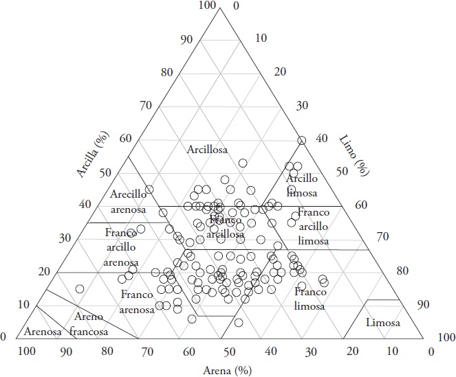
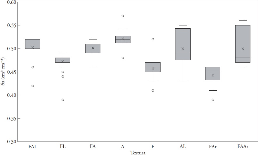
The moisture content at saturation was variable between plots, even in the same textural class, which is why the calculation of the optimal irrigation flow rate with an average value can give different results. Thus, it is convenient to obtain the experimental measure (Figure 2).
Evaluation of irrigation tests
In the study plots, irrigation was observed with lengths from six to 119 furrows and the variation depended on the entry flow rate to the plot, which ranged between 4 and 142 L s-1. The tests in the same textural class showed different results (Table 2). The surface of irrigation test was sown with maize (Zea Mayz) (29.42 %), sorghum (Sorghum vulgare) (16.75 %), alfalfa (Medicago sativa) (16.45 %), bean (Phaseolus vulgaris) (15.12 %), jicama (Pachyrhizus erosus) (8.79 %), barley (Hordeum vulgare) (5.27 %), onion (Allium cepa) (4.35 %), and wheat (Triticum aestivum) (3.84 %).
Table 2 Results from the evaluation of the irrigation tests per textural class.
| Textura | Q(L s -1 ) | K s (cm h-1) | h f (cm) | S (%) | b (m) | |||||
|
|
σ |
|
σ |
|
σ |
|
σ |
|
σ | |
| A | 50.74 | 22.02 | 1.86 | 1.25 | 110.64 | 36.20 | 0.27 | 0.18 | 0.79 | 0.11 |
| AL | 51.14 | 23.31 | 1.25 | 0.77 | 116.00 | 36.95 | 0.41 | 0.09 | 0.78 | 0.04 |
| F | 40.84 | 28.44 | 1.33 | 0.90 | 74.17 | 33.73 | 0.19 | 0.10 | 0.82 | 0.14 |
| FAAr | 50.06 | 16.35 | 1.95 | 0.93 | 103.64 | 51.96 | 0.18 | 0.14 | 0.85 | 0.05 |
| FAL | 57.28 | 19.66 | 1.75 | 1.09 | 75.84 | 35.70 | 0.20 | 0.14 | 0.86 | 0.23 |
| FA | 51.88 | 28.38 | 1.74 | 1.26 | 72.55 | 33.46 | 0.18 | 0.12 | 0.81 | 0.07 |
| FAr | 38.62 | 25.61 | 1.92 | 1.11 | 67.39 | 33.72 | 0.19 | 0.10 | 0.82 | 0.04 |
| FL | 50.48 | 23.20 | 1.62 | 1.37 | 86.66 | 39.11 | 0.17 | 0.09 | 0.80 | 0.08 |
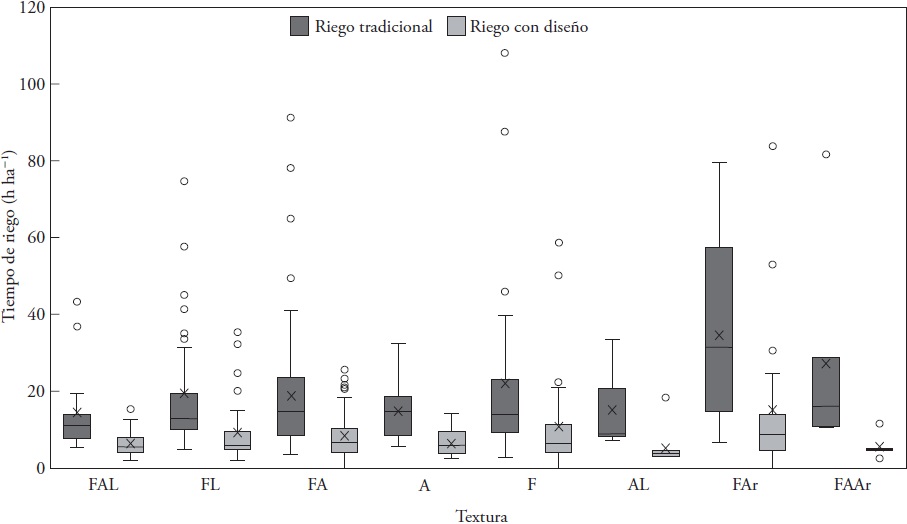
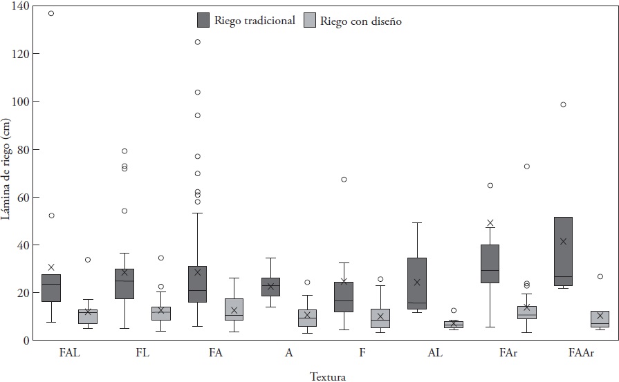
The average efficiency of application was 53 %; however, in some cases it was lower than 20 %. In the soils with higher sand content, the irrigation time was higher than in those where clays predominated (Figure 3). The atypical points in the graph correspond to plots with irrigation lengths over 130 m. The water depths applied were higher, about 15 cm, to those recommended, since the average was 30.31 cm, although in some cases water depths measured up to 138 cm (Figure 4).
Irrigation design with the optimal flow rate formula
In all the textural classes there was a considerable reduction in the number of furrows per length (Figure 5). In the most critical case, it went from 105 to 39 furrows per length, since in that plot to irrigate 1 ha the entry flow rate was 38.85 L s-1 for 57.3 h. After the recommendation, the time was reduced to 12.97 h, which was equivalent to using in the traditional case a volume of 7 972.02 m3 and with the recommendation, 1 814.4 m3; the savings was 6 157.62 m3 ha-1 in each irrigation event.
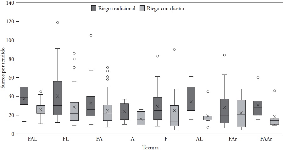
Figure 5 Furrows per length of conventional irrigation and with the analytical formula for the plot flow rates provided by the modules.
After applying the optimal flow rate to the plot, the irrigaiton times decreased in average 11.76 h ha-1 per irrigation event, although in some cases, the reduction was 61.69 h (Figures 3 and 4). The irrigation depths decreased in average 19.63 cm, and in some cases the water depth that ceased to be applied was 124.68 cm. According to the design formula, for the plots with length of more than 150 m, the optimal flow rates were higher than 4 L s-1 per furrow. These flow rates are inviable in the field because they erode the furrows, which do not have the capacity for leading them. Because of this, in these cases it was recommended to shorten the length of irrigation to around 100 m.
Volume saved
In average, 2 000 m3 ha-1 ceased to be applied. However, in some groups of sandy loam and sandy clay loam textures the saving was higher (Figure 6).

The volume that was applied in the 749.37 ha, per irrigation event, was 2.1846 million m3. With the irrigation design, the volume (1.1339 million m3) decreased 48 %. The saving of 1.0507 million m3 per irrigation, in the three average irrigation events that producers apply per cycle, is equivalent to 3.1513 million m3 in the 749.37 ha. The average irrigation efficiency achieved in the zone was higher than 85 %, which is equivalent to slightly over 30 % of the efficiency with which the users were irrigating (53 %).
Conclusions
The analytical formula for the design of optimal flow rate allows reducing the irrigation times and the highest impact is the reduction in the amount of water extracted from the storage sources. The results with this formula are a function of the characteristics of the plot (length of irrigation, slope, moisture contents, porosity and texture), and of the evaluation of the irrigation tests.
The analytical and numerical models are tools for decision making; however, the characterization of the study zone is necessary because the usefulness of the models depends on it. The average values per textural class should be taken with caution because the physical parameters and the design of the optimal flow rate are different, even within each textural class.
Literatura Citada
Banti, M., Th. Sissis, y E. Anastasiadou-Partheniou. 2011. Furrow irrigation advance simulation using a Surface-subsirface interaction model. J. Irrig. Drain. Eng. 137: 304-314. [ Links ]
Fuentes, C., B. de León-Mojarro, y F. R. Hernández-Saucedo. 2012. Hidráulica del riego por gravedad. In: Fuentes, C. y L. Rendón (eds). Riego por Gravedad. Ed. Universidad Autónoma de Querétaro, México. pp: 1-60. [ Links ]
Fuentes, C., B. De León, H. Saucedo, J.-Y. Parlange, y A.C.D. Antonino. 2004. El sistema de ecuaciones de Saint Venant y Richards del riego por gravedad: 1. La ley potencial de resistencia hidráulica. Ing. Hidrául. Méx. 19: 65-75. [ Links ]
González-Camacho, J. M., B. Muñoz-Hernandez, R. Acosta-Hernandez, y R., J. C. Mailhol. 2006. Modelo de la onda cinemática adaptado al riego por surcos cerrados. Agrociencia 40: 731-740. [ Links ]
Gillies, M. H. y R. J. Smith. 2015. SISCO: surface irrigation simulation, calibration and optimisation. Irrig. Sci. 33: 339-355. [ Links ]
Litrico, X. 2001. Nonlinear diffusive wave modeling and identification of open channels. J. Hydr. Eng. 127: 313-320. [ Links ]
Moré, J. J. 1978. The Levenberg-Marquardt algorithm: implementation and theory. In: G.A. Watson (ed). Numerical Analysis. Springer, Berlin Heidelberg. pp: 105-116. [ Links ]
Morris M. R., A. Hussain, M. H. Gillies, and N. J. O’Halloran. 2015. Inflow rate and border irrigation performance. Agric. Water Manag. 155: 76-86. [ Links ]
Rendón, L., H. Saucedo, y C. Fuentes. 2012. Diseño del riego por gravedad. In: Fuentes, C. y L. Rendón (eds). Riego por Gravedad. Ed. Universidad Autónoma de Querétaro, México. pp 321-358. [ Links ]
Saucedo, H., C. Fuentes, y M. Zavala. 2005. El sistema de ecuaciones de Saint-Venant y Richards del riego por gravedad: 2. Acoplamiento numérico para la fase de avance en el riego por melgas. Ing. Hidrául. Méx. 20: 109-119. [ Links ]
Saucedo, H., M. Zavala, y C. Fuentes. 2011. Modelo hidrodinámico completo para el riego por melgas. Tecnol. Cien. Agua 2: 23-38. [ Links ]
Saucedo, H., M. Zavala, y C. Fuentes. 2015. Diseño de riego por melgas empleando las ecuaciones de Saint-Venant y Green y Ampt. Tecnol. Cien. Agua 6: 103-112. [ Links ]
Seidel S.J., N. Schutze, M. Fahle, J.-C Mailhol, and P. Ruelle. 2015. Optimal irrigation scheduling, irrigation control and drip line layout to increase water productivity and profit in subsurface drip-irrigated agriculture. Irrig. Drain. 64: 501-518. [ Links ]
Sotelo A.G. 1977. Hidráulica General: Fundamentos. Ed. Limusa, México. 551 p. [ Links ]
Woolhiser, D. A. 1975. Simulation of unsteady overland flow. In: Mahmood, K., and V. Yevjevich (eds). Unsteady Flow in Open Channels vol. II. Water Resources Publications, Fort Collins, Colorado. pp: 485-508. [ Links ]
Received: February 2017; Accepted: July 2017
 Este es un artículo publicado en acceso abierto bajo una licencia
Creative Commons
Este es un artículo publicado en acceso abierto bajo una licencia
Creative Commons
