


Servicios Personalizados
Revista
Articulo
 texto en
  Inglés (pdf)
 Artículo en XML
 Referencias del artículo
 Enviar artículo por email
Indicadores
-
 Citado por SciELO
 -
 Accesos
Links relacionados
-
 Similares en
SciELO
Similares en
SciELO
Compartir

 Permalink
Revista ALCONPAT
versión On-line ISSN 2007-6835
Rev. ALCONPAT vol.6 no.2 Mérida may./ago. 2016
https://doi.org/10.21041/ra.v6i2.137
Basic research
A new model for the design of rectangular combined boundary footings with two restricted opposite sides
1 Facultad de ingeniería, Ciencias y Arquitectura. Universidad Juárez del Estado de Durango, Gómez Palacio, Durango, México.
This document presents a new model for the design of rectangular combined boundary footings with two restricted opposite sides, taking into consideration the real pressure of the ground on the contact surface of the footing in order to obtain: the moments around the longitudinal axes parallel to axis “Y-Y”; the moments around the transversal axes parallel to the “X-X” axis; the unidirectional shear force (Flexural shearing); and the bi-directional shear force (penetration shearing) for the two columns. The real pressure of the ground is presented in terms of the mechanical elements that act on each column (P, Mx, and My). The mathematical approach suggested in this work gives results with a tangible preciseness in order to find the most economical solution.
Keywords: footing design; rectangular combined boundary footings; moments; unidirectional shearing force (flexural shearing); bi-directional shearing force (penetration shearing)
Este documento presenta un nuevo modelo para diseño de zapatas combinadas rectangulares de lindero con dos lados opuestos restringidos tomando en cuenta la presión real del suelo sobre la superficie de contacto de la zapata para obtener: Los momentos alrededor de ejes longitudinales paralelos al eje “Y-Y”; Los momentos alrededor de ejes transversales paralelos al eje “X-X”; La fuerza cortante unidireccional (Cortante por flexión); La fuerza cortante bidireccional (cortante por penetración) para las dos columnas. La presión real del suelo se presenta en función de los elementos mecánicos que actúan en cada columna (P, Mx, y My). El enfoque matemático sugerido en este trabajo produce resultados que tienen una exactitud tangible para encontrar la solución más económica.
Palabras clave: diseño de zapatas; zapatas combinadas rectangulares de lindero; momentos; fuerza cortante unidireccional (cortante por flexión); fuerza cortante bidireccional (cortante por penetración)
Este trabalho apresenta um novo modelo de projeto de sapatas associadas retangulares de divisa com dois lados opostos restringidos, tendo em conta a pressão real do solo na superfície de contato da sapata para obter: os momentos em torno dos eixos longitudinais paralelos ao eixo “Y-Y”; os momentos em torno eixos transversais paralelos ao eixo “X-X”; A força cortante unidirecional (cortante por flexão); A força cortante bidirecional (puncionamento) para os dois pilares. A pressão real do solo é apresentada em termos de elementos mecânicos que atuam em cada pilar (P, Mx, e My). A abordagem matemática sugerida neste trabalho produz resultados que têm uma precisão tangível para encontrar a solução mais econômica.
Palavras-chave: projeto de sapatas; sapatas associadas retangulares de divisa; momentos; força cortante unidirecional (cortante por flexão); força cortante bidirecional (puncionamento)
1.Introduction
The substructure or foundation is the part of the structure that is generally placed underneath the surface of the plot of land and which transfers the loads to the ground or to the subjacent rock. Each construction requires solving a foundation problem. Foundations are classified as shallow or deep, which represent the important differences in accordance with their geometry, in terms of the behavior of the ground, their structural use, and their constructive systems (Bowles, 1996; Nilson, 1999; Das et al., 2006).
Shallow foundations, whose constructive systems generally do not present major difficulties, can be of different types depending on their use: isolated footing, combined footing, strip footing, or foundation slab (Bowles, 1996; Das et al., 2006).
The normal work of the structural analysis is normally done with the hypothesis that the structure of the buildings is embedded on the floor, i.e., it is supported by an un-deformable material (Calavera-Ruiz, 2000; Tomlinson, 2008).
The distribution of the pressure of the ground under a footing is a function of the type of soil, the relative rigidity of the soil and the foundation, and the depth of the foundation at the contact level between the footing and the ground. One concrete footing resting on thick granular soils (sandy soils) will have a similar pressure distribution as the one shown in Figure 1(a). When a rigid footing is resting on sandy soil, the sand near the borders of the footing tends to move laterally when the footing is loaded, this tends to decrease the pressure of the soil near the borders while the soil far from the borders of the footing is relatively confined. In contrast, the distribution of pressure under one footing that lies on fine-grained soils (clay soil) is similar to Figure 1(b); when the footing is loaded, the soil under the footing is deviated in a bowl-shaped depression, relieving the pressure under the center of the footing. For design purposes, it is common to assume that the pressure of the soil is lineally distributed. The distribution of the pressure will be uniform if the center of the footing coincides with that resulting from the applied loads, as shown in Figure 1(c) (Bowles, 1996; Nilson, 1999).
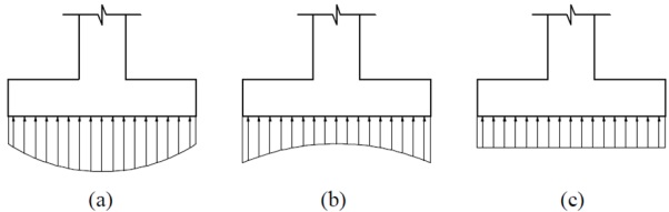
Figure 1 Distribution of the pressure under the footing: (a) Footing on thick granular soils; (b) Footing on fine soils; (c) Uniform equivalent distribution.
A combined footing is a large footing that supports two or more columns in (typically two) one row (Kurian, 2005; Punmia et al., 2007; Varghese, 2009).
Combined footings are used when: 1) The existing relation between loads, permissible capacity of the soil in the foundation, and the distance between adjacent columns make the construction of isolated footings impossible. 2) An external column is so close to the boundary of the property that it is not possible to center an isolated footing underneath it (Nilson, 1999; Kurian, 2005; Punmia et al., 2007; Varghese, 2009).
Combined footings are designed so that the centroid of the area of the footing coincides with that resulting from the loads of the two columns. This produces a uniform contact pressure on the entirety of the area and prevents the tilting tendency of the footing. On a plan view, these footings are rectangular, trapezoidal or in T-shape, and the details of their shape accommodate themselves so that they coincide with their centroid and that of the resultant (Nilson, 1999; Kurian, 2005; Punmia et al., 2007; Varghese, 2009).
Another resource used when it is not possible to center a simple footing under an external column, consists on placing the footing for the external column in an eccentric manner and connect it to the footing of the closest internal column through a beam or a supporting band. This support beam, when balanced by the load of the internal column, can resist the tilting tendency of the eccentric external footing and matches all the pressures under it. This type of foundations is known as footing with support beams, projected or connected (Nilson, 1999; Kurian, 2005; Punmia et al., 2007; Varghese, 2009).
Another solution for the design of the combined footings under columns subjected to biaxial-flexure is to consider the maximum pressure of the ground, which is considered uniform at all points of contact (Calavera-Ruiz, 2000; Tomlinson, 2008).
Some recently published documents that consider the real pressure of the ground are: Design of rectangular-shaped isolated footings using a new model (Luévanos-Rojas et al, 2013); Design of circular-shaped isolated footings using a new model (Luévanos-Rojas, 2014a); Design of rectangular-shaped combined boundary footings using a new model (Luévanos-Rojas, 2014b), this footing considers only one restricted side.
This document presents a new model for the design of rectangular combined boundary footings with two restricted opposite sides to obtain: 1) The moments around a longitudinal axis (one a-a axis with a “b1” width and a b-b axis with a “b2” width, which are parallel to the “Y-Y” axis; 2) The moments around a transversal axis (one c-c axis, one d-d axis, and one e-e axis that are parallel to the “X-X” axis); 3) The unidirectional shear force (Flexural shearing) on the f-f, g-g, h-h, and i-i axes; 4) The bidirectional shear force (Shearing by penetration) on a rectangular section formed by points 5, 6, 7, and 8 for column 1 (left boundary) and the rectangular section formed by points 9, 10, 11, and 12 for column 2 (right boundary). The real pressure of the ground that acts on the contact surface of the footing is different on the four corners, this pressure is presented in terms of the mechanical elements that act on each column (axial load, moment around the “X” axis, and moment around the “Y” axis). The mathematical approach suggested in this work produces results that have a tangible precision for all the problems, which is an essential part of this investigation to find the most economical solution.
2. Proposed model
2.1 General considerations
According to the requirements of the Construction Code for Structural Concrete and Comments, the critical sections are: 1) the maximum moment is found on the face of the column, pedestal, or wall for footings that support a concrete column, pedestal, or wall; 2) the flexural shear force is presented at a “d” distance (distance from the extreme compressed fiber to the center of the longitudinal reinforcement steel) and will be measured from the face of the column, pedestal, or wall for footings that support a column, pedestal, or on the wall; and 3) the shear force by penetration is located so that the “bo” perimeter is a minimum, but should not come closed to less than “d/2” to: (a) the borders or corners of the columns, the concentrated loads, or reaction zones; and (b) the changes in the thickness of the slab, such as the borders of the capitals, abacus, or cutting cover (ACI, 2013; McCormac y Brown, 2013).
The general equation for any type of footings subject to bidirectional flexion is (González-Cuevas y Robles-Fernández-Villegas, 2005; Punmia et al., 2007; Gere and Goodo, 2009):
where:
σ: pressure exercised by the ground on the footing (pressure of the plot of land),
A: contact area of the footing,
P: e axial load applied on the center of gravity of the footing,
Mx: moment around the “X” axis,
My: moment around the “Y” axis,
x: distance in the “X” direction measured from the “Y” axis to the fiber in the study,
y: distance in the “Y” direction measured from the “X” axis to the fiber being studied,
Iy: moment of inertia around the “Y” axis,
Ix: moment of inertia around the “X” axis.
2.2. Model for the dimensioning of the footings
Figure 2 shows a rectangular combined boundary footing with two restricted opposite sides supporting two rectangular columns of different dimensions, each column subject to an axial load and moment in two directions (bidirectional flexure).
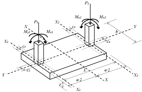
The value of “a” is fixed and can be expressed in terms of “L” as follows:
where: a is the dimension of the footing parallel to the “Y” axis.
Replacing A = ab, Ix = ba3 /12, Iy = ab3 /12, y = a/2, x = b/2 in the equation (1) we obtain:
where:
b: dimension of the footing parallel to the “X” axis,
R= P1 +P2, My T = My1 +My2 : total moment around the “Y” axis,
Mx T = Mx1 +Mx2 + P1 (a/2-c1 /2)-P2 (a/2-c3 /2): total moment around the “X” axis.
Considering that the pressure of the plot of land should be zero, as the soil is not capable of resisting traction, the value of “b” is:
Considering that the pressure of the plot of land should be the permissible load capacity available of the ground “σadm”, the value of “b” is:
The permissible load capacity of the ground is obtained in the following manner:
where: qa is the permissible load of the ground, γppz is the weight of the footing, γpps is the weight of the filling of the ground.
2.3. New model for the design of footings
Figure 3 shows the pressure diagram for rectangular combined boundary footings with two restricted opposite sides subject to an axial load and the moment in two directions (bidirectional flexure) in each column, wherein the pressure is presented differently in the four corners and lineally varying throughout the length of the contact surface.
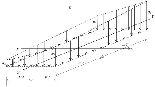
Figure 3 Pressure diagram for the rectangular combined boundary footing with two restricted opposite sides.
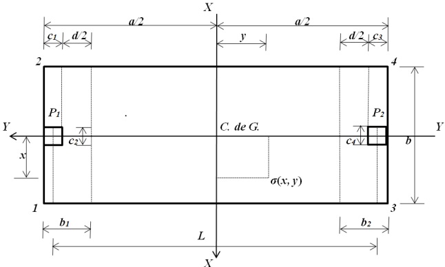
Figure 4 shows a couple of rectangular combined boundary footings with two restricted opposite sides to obtain the pressure at any place of the contact surface of the structural member due to the pressure exerted by the ground.
The pressure of the plot of land in the transversal direction is:
For column 1 it is:
For column 2 it is:
The pressure of the plot of land in the longitudinal direction is:
where: b1 = c1 + d/2 is the width of the fault surface under column 1, while b2 = c3 + d/2 is the width of the fault surface under column 2.
2.3.1. Moments
The critical sections for the moments are shown in Figure 5. These are present in sections a-a, b-b, c-c, d-d, and e-e.
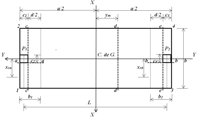
2.3.1.1. Moments around the “a-a” axis
The resulting force of “FRa” can be found through the pressure volume of the zone formed by the a-a axis with a width of b1 = c1 + d/2 and the free end of the rectangular footing, where most of the pressure is:
Now the center of gravity “xca” is obtained:
The moment around the “a-a” axis can be found through the following equation:
Replacing equations (10) and (11) in equation (12), we obtain the following:
2.3.1.2. Moments around the “b-b” axis
The resulting “FRb” force can be found through the volume of pressure of the zone formed by the b-b axis with a width of b2 = c3 + d/2 and the free end of the rectangular footing, where the most pressure is:
Now, the gravity center “xcb” is obtained:
The moment around the “b-b” axis can be found through the following equation:
Replacing equations (14) and (15) in equation (16), we obtain the following:
2.3.1.3. Moments around the “c-c” axis
The resulting “FRc” is the pressure volume of the area formed by the c-c axis and corners 1 and 2, this is presented as follows:
The center of gravity “ycc” of the pressure volume of the area formed by the c-c axis and corners 1 and 2 is obtained as follows:
The moment around the “c-c” axis is found through the following equation:
Replacing equations (18) and (19) in equation (20), we obtain the following:
2.3.1.4. Moments around the “d-d” axis
First of all, the position of the d-d axis needs to be located, as it is here where we find the maximum moment. When the shearing force has a value of zero, the moment is a maximum, thus the force “Vy = FRd - P1 ” at a “ym” distance is shown in the following manner:
The shear force “Vy” becomes zero and the value of “ym” is obtained:
The center of gravity “ycd” of the pressure volume of the area formed by the d-d axis and corners 1 and 2 is obtained as follows:
The moment around the “d-d” axis can be found through the following equation:
Replacing equations (22) and (24) in equation (25), we obtain the following:
2.3.1.5. Moments around the “e-e” axis
The resulting force “FRe” is the pressure volume of the area formed by the d-d axis and corners 1 and 2, this is presented as follows:
The center of gravity “yce” of the pressure volume of the area formed by the e-e axis and corners 1 and 2 is obtained as follows:
The moment around the “e-e” axis can be found with the following equation:
Replacing equations (27) and (28) in equation (29), we obtain the following:
2.3.1.6. Equation of moments between the two columns
To obtain the equation of moments between the two columns, it is known that the derivative of the moment is the shear force and thus it is presented as follows:
where: My is the moment at a “y” distance, and Vy is the shear force at a “y” distance.
The equation of the shear force is:
Replacing equation (32) in equation (31) and developing the integral, we obtain the following:
To evaluate the integration constant “C”, the following are replaced: y = a/2-c1 and Mc-c which appears in equation (21). The value of the constant is shown as follows:
Replacing equation (34) in equation (33), the equation of moments is obtained as follows:
2.3.2. Unidirectional shear force (flexural shearing)
The critical section for the unidirectional shear force is obtained at a distance “d” from the edge of the column, as shown in Figure 6; this is shown for sections f-f, g-g, h-h e i-i.
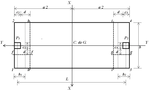
2.3.2.1. Shear force on the “f-f” axis
The flexural shear force “Vff-f” that acts on the f-f axis of the footing can be found through the pressure volume of the area formed by the f-f axis with a width of “b1 = c1 + d/2” and the free end of the rectangular footing, where most of the pressure is:
2.3.2.2. Shear force on the “g-g” axis
The flexural shear force “Vfg-g” that acts on the g-g axis of the footing can be found through the pressure volume of the area formed by the g-g axis with a width of “b2 = c3 + d/2” and the free end of the rectangular footing, where most of the pressure is:
2.3.2.3. Shear force on the “h-h” axis
The flexural shear force “Vfh-h” that acts on the h-h axis of the footing is the “P1” force that acts on column 1 minus the pressure volume of the area formed by the h-h axis and corners 1 and 2 of the footing, and is shown as follows:
2.3.2.4. Shear force on the “i-i” axis
The flexural shear force “Vfi-i” that acts on the i-i axis of the footing is the “P1” force that acts on column 1 minus the pressure volume of the area formed by the i-i axis and corners 1 and 2 of the footing, and it is shown as follows:
2.3.3. Bidirectional shear force (penetration shearing)
The critical section for the bidirectional shear force appears at a “d/2” distance from the edge of the column in both directions, as shown in Figure 7.
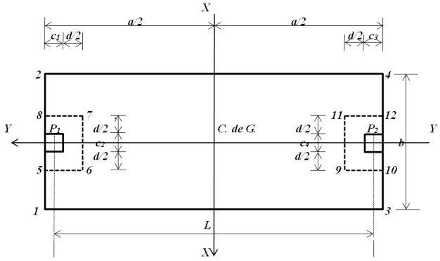
2.3.3.1. Penetration shear force for column 1
The penetration shear force of column 1 “Vp1” that acts on the footing is the “P1” force minus the rectangular area formed by points 5, 6, 7, and 8 as is shown below:
2.3.3.2. Penetration shear force for column 2
The penetration shear force of column 2 “Vp2” that acts on the footing is the “P2” force minus the rectangular area formed by points 9, 10, 11, and 12 as is shown below:
3.Numeric example
The design of a combined boundary footing with two restricted opposite sides that supports two square columns is shown in Figure 2, along with the following basic information : Column 1 = 40x40 cm; Column 2 = 40x40 cm; L = 5.60 m; H = 2.0 m; PD1 = 600 kN; PL1 = 400 kN; MDx1 = 140 kN-m; MLx1 = 100 kN-m; MDy1 = 120 kN-m; MLy1 = 80 kN-m; PD2 = 500 kN; PL2 = 300 kN; MDx2 = 120 kN-m; MLx2 = 100 kN -m; MDy2 = 110 kN-m; MLy2 = 90 kN-m; f’c = 21 MPa; fy = 420 MPa; qa = 220 kN/m2; γppz = 24 kN/m3; γpps = 15 kN/m3.
Where: H is the depth of the footing, PD is the dead load, PL is the live load, MDx is the moment around the “X-X” axis of the dead load, MLx is the moment around the “X-X” axis of the live load, MDy is the moment around the “Y-Y” axis of the dead load, and MLy is the moment around the “Y-Y” axis of the live load.
The design is done using the criterion of last resistance, and is obtained through the procedure used by Luévanos-Rojas (2014b).
Step 1: The loads and moments that act on the ground are: P1 = 1000 kN; Mx1 = 240 kN-m; My1 = 200 kN-m; P2 = 800 kN; Mx2 = 220 kN-m; My2 = 200 kN-m; R = 1800 kN; MyT = 400 kN-m; MxT = 1020 kN-m.
Step 2: The available load capacity of the ground: a thickness “t” of the footing is proposed, the first proposal is a minimum thickness of 25 cm in accordance with the ACI regulation; subsequently, the thickness is revised to comply with the conditions: moments, flexural shearing, and penetration shearing. If these conditions are not complied with, a greater thickness is proposed until the three aforementioned conditions are met. The thickness of the footing that complies with the three conditions mentioned above is of 85 cm. Using equation (6) the available load capacity of the ground is obtained “σadm”, which is of 182.35 kN/m2.
Step 3: The value of “a” by equation (2) is obtained as: a = 6.00 m. The value of “b” by equation (4) is obtained as: b = 3.08 m, and by equation (5) it is obtained as: b = 3.25 m. Therefore, the dimensions of the footing are: a = 6.00 m and b = 3.30 m.
Step 4: The mechanical elements (P, Mx, My) that act on the footing are factorized: Pu1 = 1360 kN; Mux1 = 328 kN-m; Muy1 = 272 kN-m; Pu2 = 1080 kN; Mux2 = 304 kN-m; Muy2 = 276 kN-m; R = 2440 kN; MuyT = 548 kN-m; MuxT = 1416 kN-m.
Step 5: The moments that act on the footing. The moments around the axes parallel to the Y-Y axis are: Ma-a = 544.64 kN-m; Mb-b = 457.08 kN-m. The moments around the axes parallel to the X-X axis are: Mc-c = ‒549.43 kN-m; Md-d = ‒1652.53 kN-m; Me-e = +102.49 kN-m.
Step 6: The effective depth (effective cant). The effective cant for the maximum moment of the axes parallel to the Y-Y axis is: d = 37.61 cm. The effective cant for the maximum moment of the axes parallel to the X-X axis is: d = 31.95 cm. The effective depth after different proposals is: d = 77.00 cm, r = 8.00 cm, t = 85.00 cm.
Step 7: The flexural shear force (unidirectional shear force). The shear forces in the axes parallel to the Y-Y axis, the permissible flexural shear force is: ∅v Vcf = 400.26 kN; the acting flexural shear forces are: Vff-f = 361.15 kN; Vfg-g = 304.64 kN. Therefore, it complies. The shear forces on the axes parallel to the X-X axis, the permissible flexural shear force is: ∅v Vcf = 1682.60 kN; the acting flexural shear forces are: Vfh-h = 1176.23 kN; Vfg-g = ‒ 826.48 kN. Therefore, it complies.
Step 8: The penetration shear force (bidirectional shear force). The permissible penetration shear force is: ∅v Vcp = 4191.22 kN; ∅v Vcp = 7114.75 kN; ∅v Vcp = 2711.96 kN. The acting penetration shear force is: for column 1: Vcp1 = 1189.73 kN; for column 2: Vcp2 = 1023.91 kN. Therefore, it complies.
Step 9: The reinforcing steel. w = 0.0425.
-
The longitudinal reinforcing steel (reinforcing steel in the direction of the “Y” axis).
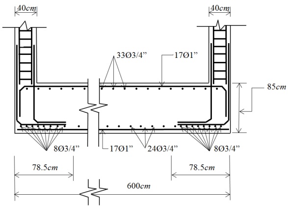
Reinforcing steel in the upper part: Asp = 58.35 cm2. Asmin = 84.62 cm2. Therefore, minimum steel by flexure is suggested “Asmin”. Use 17 rods of 1” (2.54 cm) in diameter.
The reinforcing steel in the lower part: Asp = 3.53 cm2. Asmin = 84.62 cm2. Therefore, mínimum steel by flexure is suggested “Asmin”. Use 17 rods of 1” (2.54 cm) in diameter.
-
The transversal reinforcing steel (reinforcing steel in the direction of the “X” axis):
The reinforcing steel in the lower part: Under column 1: Asp = 19.45 cm2. Asmin = 20.13 cm2. Therefore, minimum steel by flexure is suggested “Asmin”. Use 8 rods of 3/4” (1.91 cm) in diameter. Under column 2: Asp = 16.22 cm2. Asmin = 20.13 cm2. Therefore, minimum steel by flexure is suggested “Asmin”. Use 8 rods of 3/4” (1.91 cm) in diameter.
The reinforcing steel in the excess part of the columns: Steel by temperature is suggested: Ast = 0.0018bwt = 67.78 cm2 . Use 24 rods of 3/4” (1.91 cm) in diameter.
Reinforcing steel in the upper part: Steel by temperature is suggested: Ast = 0.0018bwt = 91.80 cm2. Use 33 rods of 3/4” (1.91 cm) in diameter.
Step 10: The longitude of the development for corrugated bars:
a)Reinforcing steel in the upper part where: ψt = 1.3 as it has more than 30 cm of fresh concrete under the reinforcement, ψe = λ = 1.
The available length in the longitudinal direction of the footing is: 300 - 50.19 - 8 = 241.81 cm.
Thus, the developmental length is lower than the available length. Therefore, a hook is not required.
b)Reinforcing steel in the lower part where: ψt = 1, ψe = λ = 1.
The available length in the longitudinal direction of the footing is: 330/2 - 40/2 - 8 = 137 cm. Therefore, the developmental length is lower than the available length. Therefore, a hook is not required. The dimensions and the reinforcing steel of the rectangular boundary footing that supports two square columns with two restricted opposite sides are shown in Figure 8.
4. Conclusions
The model presented in this document is only applicable for the design of rectangular combined boundary footings with two restricted opposite sides that support two columns. It is assumed that the ground under the footing is of an elastic and homogeneous material, and that the footing is rigid, which complies with the expression of the bidirectional flexure, meaning, the variation of the pressure is linear.
The equations proposed directly offer the dimensions in the layout of the foundation, guaranteeing that the permissible pressure in the ground will not be exceeded. On the other hand, the mechanical elements for moments, flexural shear force (unidirectional shear force), and penetration shear force (bi-directional shear force) can also differ from the ones obtained with a constant ground pressure. In this work, we also propose expressions to obtain these design elements in a systematic manner.
The model proposed in this document can be applied to the three types of rectangular combined boundary footings with two restricted opposite sites in terms of the loads applied to each column: 1) concentric axial load, 2) Axial load and moment in one direction (unidirectional bending), 3) Axial load and moment in two directions (bidirectional bending).
Suggestions for future investigations: 1) When the rectangular combined boundary footings with two restricted opposite sides support more than two columns; 2) When another type of soil is present, for example, in the case of completely cohesive soils (clay soils) and completely granular soils (sandy soils), the pressure diagram is not linear and they must be treated in a different manner (Figure 1); 3) In the event that only a portion of the base of the foundation generates compression on the ground, with only a portion of its contact surface working-which is allowed in some hypotheses of infrequent loads, especially in the foundations of industrial equipment, the solution of which is iterative (Bowles, 1970).
Referencias
ACI (2013), Building Code Requirements for Structural Concrete and Commentary, (New York, USA: American Concrete Institute, Committee 318). [ Links ]
Bowles, J. E. (1970), “Engineering properties of soils and their measurement”, (New York, USA: McGraw-Hill). [ Links ]
Bowles, J. E. (1996), “Foundation analysis and design”, (New York, USA: McGraw-Hill). [ Links ]
Calavera-Ruiz, J. (2000), “Cálculo de estructuras de cimentación”, (Distrito Federal, México: Intemac ediciones). [ Links ]
Das, B. M., Sordo-Zabay, E., Arrioja-Juárez, R. (2006), “Principios de Ingeniería de Cimentaciones”, (Distrito Federal, México: Cengage Learning Latín América). [ Links ]
Gere, J. M., Goodo, B. J. (2009), “Mecánica de materiales”, (Distrito Federal, México: Cengage Learning). [ Links ]
González-Cuevas, O. M., Robles-Fernández-Villegas, F. (2005), “Aspectos fundamentales del concreto reforzado”, (Distrito Federal, México: Limusa). [ Links ]
Kurian, N. P. (2005), “Design of foundation systems”, (New Delhi, India: Alpha Science Int'l Ltd.). [ Links ]
Luévanos-Rojas, A., Faudoa-Herrera, J. G., Andrade-Vallejo, R. A., Cano-Alvarez, M. A. (2013), “Design of isolated footings of rectangular form using a new model”, International Journal of Innovative Computing, Information and Control, Vol. 9, No. 10, pp. 4001-4022. [ Links ]
Luévanos-Rojas, A. (2014a), “Design of isolated footings of circular form using a new model”, Structural Engineering and Mechanics, Vol. 52, No. 4, pp. 767-786. [ Links ]
Luévanos-Rojas, A. (2014b), “Design of boundary combined footings of rectangular shape using a new model”, Dyna-Colombia, Vol. 81, No. 188, pp. 199-208. [ Links ]
McCormac, J. C., Brown R. H. (2013), “Design of reinforced concrete”, (New York, USA: John Wiley & Sons). [ Links ]
Nilson A. H. (1999), “Diseño de estructuras de concreto”, (Distrito Federal, México: McGraw-Hill). [ Links ]
Punmia, B. C., Kumar-Jain, A., Kumar-Jain, A. (2007), “Limit state design of reinforced concrete”, (New Delhi, India: Laxmi Publications (P) Limited). [ Links ]
Tomlinson, M. J. (2008), “Cimentaciones, diseño y construcción”, (Distrito Federal, México: Trillas). [ Links ]
Varghese, P. C. (2009), “Design of reinforced concrete foundations”, (New Delhi, India: PHI Learning Pvt. Ltd.). [ Links ]
Received: November 28, 2015; Accepted: March 13, 2016
 Este es un artículo publicado en acceso abierto bajo una licencia Creative Commons
