


 text new page (beta)
 English (pdf)
 Article in xml format
 Article references
 Send this article by e-mail
 Cited by SciELO
  Similars in
SciELO
Similars in
SciELO 
 Permalink
1 Introduction
Image matching is one of the most difficult problems in computer vision. Indeed, it is the fundamental precursor of 3D reconstruction from a stereo pair or image sequence. Dense image matching can be cast as finding corresponding points in two or more images that correspond to the same physical point in the scene [16, 24, 13, 23, 9, 10, 21, 6].
Dense image matching is an important step of 3D reconstruction of scenes and objects. Dense image matching can be defined as the relationship between two 2D images used to construct the 3D scene. From the 2D images, dense image matching identifies corresponding points that refer the same scene point [17, 18]. Unfortunately, many problems can be detected such as occlusions, repetitive textures, illumination changes and discontinuities of disparity.
Image matching can be achieved by several techniques. It can always be cast as an optimization problem. There are two major classes: local methods and global methods. Local methods are based on correlation (SAD, SSD, ZNCC), while global methods are based on stochastic algorithms such as taby search, genetic algorithms, or simulated annealing (SA).
Several works on simulated annealing have always claimed that the SA algorithm has the fundamental property of finding the global minimum regardless of the initial configuration. While this has been shown as an asymptotic convergence towards the global minimum in infinite time, no experimental benchmarking has been achieved either to evaluate the quality of solution or to verify that a strong minimum is reached in finite time.
Using the simulated annealing algorithm in stereo matching has several problems such as initialization of the algorithm and the random number generator. The performance of the algorithm in terms of computation time and quality of disparity map depends on control parameters as well as the cooling schedule.
In this paper, we are interested in the study and evaluation of different cooling schedules in simulated annealing algorithm [4, 22, 8, 15]. Our work focuses on evaluating the results of the simulated annealing algorithm in then context of stereo matching [20, 5].
We analyze the algorithm performances by using different initializations (configuration), initial values of temperature, and different seed value for the random number generator.
2 Simulated Annealing
Initially, the system is set in an arbitrary configuration. The annealing procedure takes the system from this initial configuration to a final state through a sequence of elementary transitions:
 (1)
(1)
where E (x k ) is the energy function value at the kth iteration.
Metropolis et al. [11] proposed an algorithm to simulate the behavior of the system as the Boltzmann distribution at temperature T . The simulated annealing uses this iterative procedure to achieve a state of thermal equilibrium. Kirkpatrick et al. [7] proposed to adapt this algorithm to solve optimization problems. The energy function is replaced by the objective function to minimize.
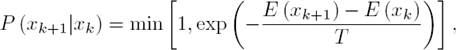
The simulated annealing algorithm starts from a random initial state and performs a random walk in the configurations space. Transitions from the current state to a new state with lower energy are always accepted. Transitions to a state with higher energy are accepted according to the Boltzmann probability distribution function: at high temperature, it is likely to accept this kind of transitions while, at low temperatures, only transitions reducing the energy are accepted. The transitions are defined according to the temperature plateaus, each plateau contains a set of configurations that could be reached at this temperature. The temperature is decreased only when the system in thermal equilibrium at the current temperature. Let assume E(x) the function to minimize. The simulated annealing algorithm is as follows:

The effectiveness of simulated annealing de-pends in the choice of certain parameters such as the initial temperature value and the cooling schedule.
2.1 Annealing Parameters
The initial temperature should not be very high to have a reasonable computation time but high enough to allow greater freedom in exploring the search space. It should not be very low to ensure convergence towards the global minimum and avoid to be trapped in local minima.
One way to choose the value of the initial temper-ature, is to generate a number of transformations and to calculate their average cost x 0. The initial temperature value of the temperature can be set as [2]:
 (2)
(2)
3 Cooling Schedule
The cooling schedule is the procedure that decreases the temperature parameter. Bringing the temperature parameter from a large value to zero too quickly has some dramatic consequences on the quality of the solution. Lowering the temperature too slowly may result in a large computation time. The speed of convergence towards the global minimum and the quality of the solution depend on the cooling schedule. We propose to study several cooling schedules available in the literature:
3.1 Logarithmic Cooling Schedule
Geman and Geman [3] defined a cooling schedule as
 (3)
(3)
where c is positive constant independent of t but depending on the problem. Theoretically, the logarithmic cooling schedule asymptotically converges towards the global minimum. However, this scheme converges very slowly and requires a large computation time.
3.2 Geometrical and Linear Cooling Schedule
This type of cooling schedule is faster than the logarithmic cooling scheme [14, 15], as it decreases geometrically
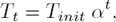 (4)
(4)
where α is a constant between 0 and 1. To have a slow decrease of temperature, it is necessary that the value of α is closer to 1.
The linear cooling schedule is defined as follows
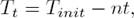 (5)
(5)
where t is the iteration number and n is the decay parameter. These strategies do not guarantee convergence towards the global optimum, but they converge more rapidly towards a strong minimum (strong minima are solutions that lie in the near vicinity of the global minimum).
3.3 Adaptive Schedule (Reversibility)
This cooling schedule slightly differs from the geometric cooling schedule [15]. It decreases the temperature when the new average energy is less than or equal to the previous average energy.
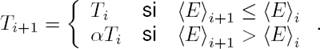 (6)
(6)
This schedule has two major drawbacks, namely the constant a must be adjusted properly and it is very slow in practice.
3.4 Arithmetic-Geometric Cooling Schedule
We also propose to consider a cooling schedule inspired by the arithmetic-geometric progression. This progression is defined as a recurrence affine relation between a term and the next term of the sequence. It is defined as
 (7)
(7)
In the case a = 1, this progression would be an arithmetic progression and when b = 0, we would have a geometric progression. Consequently, parameters a and b must be different from 1 and 0 respectively.
There are various behavior of the values that can take a:
a > 1 : The progression diverges to plus ±∞.
|a| < 1 : The progression converges to  .
.
a ≤ −1 : The progression diverges (±∞ are not necessarily limit of the progression).
4 Simulated Annealing without Cooling Schedule (WCS)
Dieter Muller has proven that we can reach the Boltzmann distribution without having to specify the temperature parameter T [12]. The proposed distribution is given by:
 (8)
(8)
 (9)
(9)
The parameter β is identical to the quantity  in the standard simulated annealing. This explains that we can achieve an approximation of the Boltzmann distribution without having to indicate the value of temperature T .
5 Microcanonical Annealing
A variant of simulated annealing is the micro-canonical annealing [1]. the main difference with simulated annealing is the convergence towards the global optimum. The first is based on plateaus of temperature and the second on decreasing plateau of total energy related to the reduction of kinetic energy at each plateau.
Microcanonical annealing algorithm implements Creutz procedure [1], which is based on the assessment of a succession of transitions to maximize the entropy for a total energy constant. This energy is fixed beforehand.

Creutz algorithm is much simpler than Metropolis algorithm and requires much less computation time. Compared with simulated annealing, in the case of large problems, several studies have shown that the results obtained are very close, with an advantage for the microcanonical annealing in terms of computation time.
The value of the kinetic energy is E D = E t − E (x k ) , E t is the total energy which is high at the beginning of the algorithm. Reducing the total energy, the algorithm will converge to the global optimum.
6 Modeling the Energy Function
The experimental study is conducted in the context of stereo matching. The computation of disparity maps is modeled as an optimization problem where the energy functional is specified according to known problem constraints. Taking into account the stereo matching in both directions (left-right and right-left), the energy function will be modeled considering the following constraints: resemblance, epipolar geometry, continuity of the disparity, and uniqueness [19, 17, 18].
6.2 Resemblance Constraint
The resemblance constraint stipulates that matched pixels should have similar gray levels, which is fundamentally true in the case of Lambertian surfaces. The constraint is defined as follows:
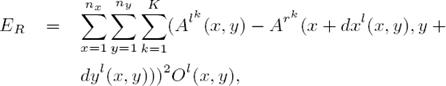 (10)
(10)
where K is the number of lighting conditions.
6.3 Continuity of the Disparity Constraint
We consider that physical surfaces are locally continuous. In this case the Euclidean projection is also continuous. Since the disparity varies smoothly, except at depth edges, the constraint is cancelled around contours, as well as occlusions. This constraint can be expressed as:

6.4 Number of Occlusions
To limit the number of occlusions in the image, we add a counterweight for the energy function. For a single image, the functional is:
 (11)
(11)
6.5 Uniqueness Constraint
A pixel can only matched with one pixel in the other image. This constraint reduces the number of possible matches, it is expressed in elementary transitions.
6.6 Epipolar Geometry
The epipolar constraint reduces the search space of corresponding to a line called the epipolar line. This allows to avoid wrong matchings and reduces computation time.
The energy functional is the weighted sum of energy functionals derived from the constraints:
 (12)
(12)
where ρ R ; ρ c ; ρ O are the energy functional terms weighting coefficients.
7 Experimentation
In this section, we analyze and evaluate the performance of different cooling schedules used in the simulated annealing algorithm and the dif-ferent variants without cooling schedule described above.
The results are evaluated by calculating the mean absolute error (MAE), the mean relative error (MRE) and the percentage of correct matches (C) as well as wrong matches (E). Other important evaluation criteria are the visual aspect of disparity maps and the computation time.
7.1 Parameters Setting
The experimentation is conducted on synthesized imagery which are illustrated in Figure 1.
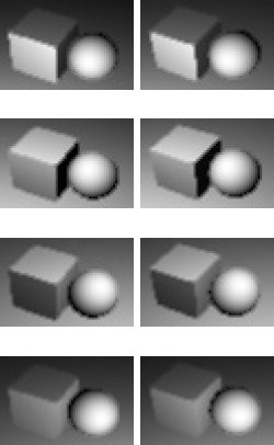
Fig. 1 The first column represents the left-hand side and the second column represents the right-hand side. Each row corresponds to particular lighting condition
Figure 1 represents the synthesized images used in this experimentation. The first column of images is the left-hand side and the second column of images is the right-hand side. These images are generated under four different lighting conditions. The images are 60 × 40.
The algorithm is initialized with disparity maps and occlusion calculated by the SAD correlation method, over 5 × 5 window. We have implemented the SAD correlation algorithm with the same stereo constrains.
The initial temperature is set to 1, 000 for all cooling schedules except the logarithm cooling schedule for which it was set to 1. This is because this schedule is very slow. For the microcanonical annealing, the total energy is equal to 70, 000.
Table 1 shows the parameters of the different cooling schedules used in this study.

The weighting coefficients of the energy function are the same as the ones defined in [17, 18] ρ R = 5; ρ O = 2; ρ C = 0.25.
The number of iterations within a temperature plateau is given by M = τ (size of domain); the parameter τ is equal to 100. These parameters have proven to give good results.
7.2 Results and Discussion
Numerical results obtained in this study for the left disparity maps are defined in the Table 2.
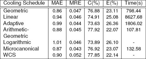
The numerical results of the right disparity maps are nearly the same and do not necessitate to be shown separately.
The analysis of the results described in Table 2 show that the cooling schedule arithmetic-geometric and WCS have produced a high per-centage of correct matches with a small advantage for arithmetic-geometric cooling schedule. We note 77.95% of correct matches produced by the arithmetic-geometric cooling schedule.
The low percentage of correct matches is recorded for adaptive cooling schedule with 73.63%.
As seen in Table 2, logarithmic cooling schedule and WCS algorithm do not have a time record because these variants are time consuming. These variants are stopping after blocking.
In Figure 2, we show the visual of stereo matching for each cooling schedule, as we observe, the simulated annealing produced some amount of occlusions.
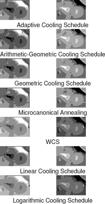
Fig. 2 The visual result of stereo matching. Disparity maps computed with different cooling schedules and variants
Figure 2 shows the disparity maps obtained by each cooling schedule. For each cooling schedule, the left image represents the disparity map of the left-right direction and the right image represents the disparity map of the right-left direction.
We observe also that the geometrical cooling schedule and microcanonical annealing produce good results in terms of computation time and produce few errors compared to other alternatives.
The arithmetic-geometric cooling schedule de-creases rapidly. Although it gave good result, this scheme could have trapped the algorithm in a local minimum.
We conducted our experiments with different initializations: disparity map from correlation, disparity map with 0 values, and initialization with synthesized solution. We also made sure the random number generator is always initially fed with a different seed point. For all these cases, we obtained a roughly similar energy value solution. The disparity maps are also almost identical, which confirms that our implementations achieve a strong minimum in finite time. Figure 3 shows the evolution of each term of the energy functional. We observe that during the first plateaus, some cooling schedules exploit the solution space by accepting the transition which increases the energy function when the temperature is very high.
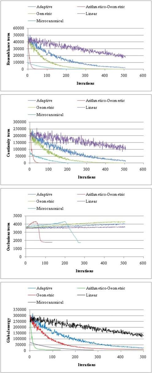
Fig. 3 This figure shows the evolution of each term of the energy functional per plateaus as well as the total energy of the system
Figure 3 illustrates the function values of each cooling schedule. Subfigure (a) shows the resemblance term, the second subfigure (b) represents the continuity term, the third subfigure (c) represents the occlusion term and the last subfigure (d) shows the global energy function.
As seen in Figure 3, we observe that the continuity and the resemblance are decreasing and converging to small values. The global energy generated by geometric cooling schedule decreases rapidly in the first 170 iterations. Thereafter, it decreases slowly.
8 Conclusion
In this paper, we have studied and analyzed the perfermances of different cooling schedules used in conjonction with the simulated annealing and other variants without cooling schedule. The experimentations were conducted in the context of stereo matching. The microcanonical annealing and the geometrical cooling schedule have proven their perfermances in matching with an advantage for microcanonical annealing which produces a small number of occlusions. The logarithmic schedule is very slow and it is unrealizable in practice. The results obtained by WCS show that this approach is also very slow.
Last but not least, regardless of the initial state, our implementation of the S.A. algorithm variants along with the cooling schedules always converges towards a strong minimum. It is important to note that the disparity maps are almost identical and the final value of the energy functional is almost the same.

