


 text new page (beta)
 English (pdf)
 Article in xml format
 Article references
 Send this article by e-mail
 Cited by SciELO
  Similars in
SciELO
Similars in
SciELO 
 Permalink
1 Introduction
It is well known that a system of stochastic differential equations describes the evolution of the prices of two or more risky assets [1]. The options derived from those two or more underlying risky assets are called multiple-asset options and can be modeled as a terminal-boundary value problem with the multi-dimensional partial differential Black-Scholes equation, in two or more variables, depending on the assets. Due to the complexity of the explicit solution of the equation mentioned above, an essential issue in the price of multiple-asset options is whether a pricing problem can be reduced to a one-dimensional problem by introducing new appropriate variables. One widely used possibility is the use of the so-called numeraire change method, which is important in reducing the number of risk sources to be considered in the price of the options, as well as gives significant computational simplifications [2,3]. A numeraire is any strictly positive price process whose choice does not change the properties of the market. It is used to compare numerical values of two different portfolios, expressing them in terms of the same numeraire [4]. The basic idea of the numeraire approach is to choose a variable that incorporates one of the risk sources and express all market prices in terms of the one chosen as the numeraire. This numeraire asset is risk-free in the new pricing system, thus reducing the number of risk factors from n to n - 1.At the end of the calculation, it is possible to return to the standard prices through a simple transformation [2]. Furthermore, in [5] authors introduce a more general multiplicative transformation which can be applied repeatedly, reducing the number of dimensions by two or more and therefore the sources of risks. They obtain a modified Black-Scholes formula for the option’s price, which depends on the volatilities of both variables.
In this paper, we propose a different strategy based not on reducing risks but on considering how much influence one variable has on the other variables. This is achieved by using a projection scheme that has been developed with great success in the study of diffusion in confined systems [6-10]. The method consists of choosing a variable, called transversal, whose influence is bounded and can depend on the other variable that is usually known as longitudinal. To apply this method clearly, we choose a two-variable system and its projection to one dimension. In particular, the evolution of the option price with an exercise price in foreign currency is studied. In this case, both the stock price and the exchange rate will be the two variables on which the option’s price will depend. As is well known for certain assumptions in the evolution of prices, it is possible to establish a relationship between the Black-Scholes equation and the usual diffusion equation. Therefore the present method will work under the same assumptions.
The paper is organized as follows: In Sec. 2 we present the general equation of Black-Scholes in two dimensions and briefly summarize the result of the generalized method for this problem which was already presented in [5]. In 3 we review the basic steps of the projection method to one dimension of the diffusion equation for a confined system proposed by Zwanzig. This gives rise to the so-called Fick-Jacobs equation, which is an effective one-dimensional diffusion equation modified by the width of the channel [6,7,9,10].
In Sec. 4 the projection method is implemented on the two-dimensional equation of Black-Scholes, obtaining first a Fick-Jacobs-like equation, where the influence of the range where the variable of the exchange rate is clearly defined. This acts as the channel width in the Fick-Jacobs equation but with extra drag and relaxation terms. To give an adequate interpretation, we rewrite that equation as an effective one-dimensional Black-Scholes equation that contains two effective parameters for the interest rates, which include the influence of the integrated variable. If the relationship between both variables is modeled as a power law, both rates depend only on the corresponding exponent, thus modulating its influence. This result contrasts with the numeraire approach or the generalized transformation where a source of risk is reduced, while here, it remains even after integrating a variable.
In Sec. 5, we solve the effective Black-Scholes equation for the value of a European call option at expiration time T and strike price Kp, obtaining an effective version of the so-called Black-Scholes formula, whose modification is due to the different interest rates and on the exponent of the power-law. Finally, we graphically compare both solutions for typical values of the variables, and we obtain that the relative error between both is bounded for short times. In the last 6, we briefly summarize the results of the work.
2 Multidimensional Black-Scholes equation and its reduction
We focus on the well-known model in financial mathematics, the so-called Black-Scholes partial differential equation, which is a very particular and important case of the diffusion model to describe the price of the options [11,12]. The option prices derived from several underlying assets satisfy the multidimensional Black-Scholes equations [1,3,5]. The (n + 1)-dimensional Black-Scholes equation is given in the following way:
where
To describe the exercise price of an option when the underlying stock is traded in one currency, and the exercise price of the option is in a different one, it is possible to use Eq. (1) in two dimensions, where one variable will be the price S(t) of the stock and the other will be the exchange rate between foreign currencies X(t). At the initial time, the exercise price is the same as the underlying stock price in the first currency. Initially, it is converted to the second currency and held for the life of the option. The problem is finding the right price at the maturity date when the holder decides whether to pay the exercise price in the second currency to buy the underlying stock. Let rp be the corresponding rate in the original currency, rd the rate in the new currency, Kd the exercise price expressed in the second currency, and Kp the first one.
By considering the same assumptions as in Ref [5], namely, S(t) follows a geometric Brownian motion, X(t) follows the Garman-Kohlhagen model [13], the rates are considered constants, and the Wiener scalar processes of each variable satisfy the following
t is possible to write a Black-Scholes equation for pricing model through the Itô formula [14]
Where V(S, X, T) is the payoff function at expiry date, and the strike price
In Ref. [5] starting from Eq. (3) by the use of a generalized transformation they could reduce problem (3)-(4) with the introduction of the group variable z = SX, to the following
where
where
and the cumulative distribution function (CDF) of a normal random variable is defined as
In the last section, we will return to expressions (7)-(36) to compare with the result obtained with the new proposal.
3 Projection method for the diffusion in confined systems
In this section, we review the reduction to one dimension introduced to study physical diffusion in quasi-unidimensional asymmetric channels.
For a 2D channel with boundaries defined by
Let us start with the diffusion equation in two dimensions for the concentration
with initial anisotropic diffusion constants
The method consists of integrating into the transversal coordinate y. So, when imposing the parallel-to-boundary-flux, as a boundary condition, and by the use of the Leibniz rule, i.e.,
it is possible to turn Eq. (10) into an equation for P(x, t). This is the so-called Fick-Jacobs equation when
It is worth noting that for this effective 1D diffusion, a drift and a relaxation term induced by the channel width w(x) can be seen when the equation is rewritten as
We will use this form of the equation later. The drift is caused by the so-called entropic force induced by the boundaries, also called entropic barriers [6].
The (13) is the lowest order in a projective method that considers that the concentration also depends on the transversal coordinate, see [7-9] for channels. We will limit ourselves to the lowest order in this work, and the complete treatment will be done elsewhere.
4 Projection method for the 2D Black-Scholes equation
Let us first define the marginal option price that only depends on the stock price by integrating what we call the transversal variable, which in this case is the exchange rate between foreign currencies X Thus, it is necessary to indicate the dependence of the price X on S. This will be modeled through function X = f(S), which is the analog of the channel width for confined systems
where we consider that the lowest exchange rate is zero, that is, without variation; of course, both the range and the explicit form of f will depend on the characteristics of each market and the different currencies. Here we will use power-law type dependencies, only to exemplify the results.
Let us integrate Eq. (3) over X in some derivative terms the use of Leibniz rule (12) is needed because the integration limits depend on S so that the final form is the following
In order to simplify this equation, we need to introduce boundary conditions in the same way as in the projection method. This is achieved when we impose that the currency exchange can not exceed the maximum of f(S), that is, when the following boundary condition is met
The following is to introduce the order of approximation. At the lowest order, price V does not depend explicitly on X, and from (15), we can write
After these considerations and some algebra where terms are reduced, (16) can be written in the following simplified form
This equation is similar to Fick-Jacobs Eq. (13) for diffusion in channels, where f is analogous to the channel’s width w and induces modifications into the differential operators. Thus, f will induce an additional drag term and also a modification to the relaxation term. This can be seen when it is written as follows
that can be interpreted as a one-dimensional effective Black-Scholes equation for the marginal price U, where the effective rates are
Comparing (20) with the reduced (5), we can note that instead of effective volatility and the interest rate in the second currency, in this case, the volatility of the stock remains but two effective rates based on rd appear, with modifications due not only to volatilities but now with a coupling to the possible dependence of X on S given by f. It is noteworthy that since f is a function of S, the induced rates will not be constant in the general case. However, if we consider a simplified model where f is a power law of the form
so the rates can be rewritten as
which become constants that only depend on the corresponding power. Note that only in the case where m = 0 and the correlation is zero, the two rates will coincide.
The next step will be to obtain the corresponding effective Black-Scholes formula for this problem with the rates r1 and r2, solving (20) and comparing with the one previously obtained in [5].
5 Effective Black-Scholes formula
As usual for the solution of this equation, the following well-known variable change is chosen, which also serves to scale the variables in dimensionless quantities
ith T the maturity time and the price function given by
With this, (20) becomes
where
with terminal condition
thus, the equation becomes
When we neglect the coefficients of the second and third term on the right side of Eq. (31), we obtain the standard dimensionless diffusion equation
The solution to the heat equation can be written in terms of the CDF of a normal random variable (9) as
where
When we return to the original variables, substituting the values of q1 and q2, we obtain the following expression that can be regarded as the effective Black-Scholes formula for our problem
where
When comparing this solution with (7), we notice is that (35) does not depend on X. The first term contains an additional temporal dependence that vanishes only when
In order to graphically compare both formulas, let us consider the value of a call option with an exercise price of Kp = 100 in the first currency. The expiration time will be at, say, one year T = 1. Taking into account the risk-free interest rate in the first coin to be rd = 0.12. For the volatilities
The relative difference
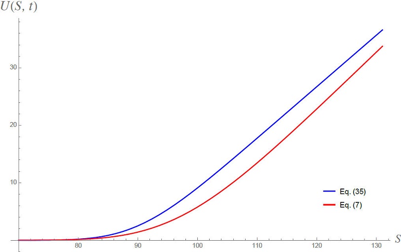
Figure 1 Value of the call option when the underlying stock price and strike price in two different currencies, both evaluated near initial time t = 0.1. Blue curve corresponds to effective Black-Scholes formula (35) with m = 1. Red curve is (7) considering X(0) = 1.3 and evaluating at Xi = 1.2.
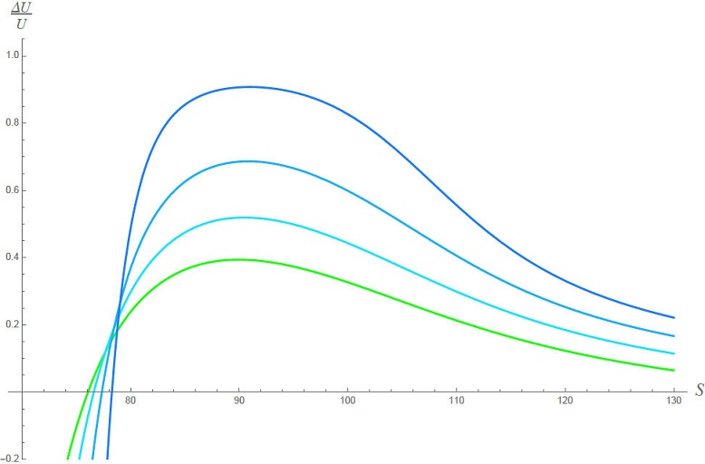
Figure 2 Relative diference of both solutions (7) and (35). The green curve is close to t = 0, while going to increasingly blue curves increases the time progressively.
Qualitatively both solutions are very similar and do not differ too much from one another. However, the comparison strongly depends on the value of X in which we are comparing. Equation (35) contains the influence of the possible dependence of S on X modeled through the function f, which is still to be established.
For instance, by varying m, it is possible to change the behavior of the price. Indeed, for a fixed value of the correlation, the variation of the exponent can be seen in Figs. 3 and 4. As m grows from 0 to 4, the growth of U becomes slower. This difference decreases as we get closer to the expiration date of the option Fig. 4. It must be determined if this can be observed in the actual behavior of the market. This will indicate the further need to obtain suitable models for f.
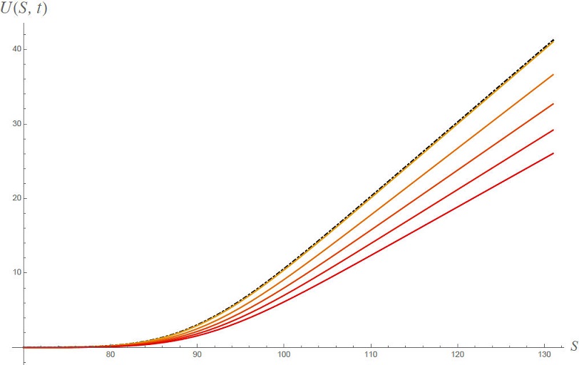
Figure 3 Call option value from (35) at t = 0. The black dot-dashed line is the case
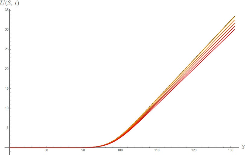
Figure 4 Call option value from Eq. (35) a t = 0.8. Colors as in Fig. 3. The effect of m decreases when approaching the expiration date of the option.
6 Conclusions
In this paper, we apply Zwanwig’s projection method, developed to study diffusion in channels, to the bidimensional Black-Scholes equation for the case in which the option’s value depends, in addition to the price of the underlying stock, on the exchange rate to a different currency. This case had already been studied by O, Ro, and Wan in Ref [5], whose solution could be written in a very similar form to a one-dimensional Black-Scholes formula but dependent on the variable of exchange rate and of effective volatility
These results open the possibility for the study of multidimensional option pricing problems. They appear when dealing with price options on various underlying assets, such as finding the price of options in a basket that is a financial instrument where the underlying asset is a portfolio of several assets, for example, individual stocks. Most of the works in several dimensions are mainly numerical, and only a few present some exact solutions and approximations [5,18], so generalizing the present results to various dimensions would be very useful. The projection method, either Zwanzig’s or its generalization by Kalinay and Percus, has been successfully applied to reduce two and three-dimensional systems by introducing the width or cross-sectional area function into an effective equation and appropriate position-dependent diffusion coefficient [7,8]. In n dimensions, it would be necessary to guarantee that the problem definition domain is such that one of the dimensions is much larger than the other n - 1 and then project towards the longitudinal variable. An alternative method to find the diffusion coefficient was proposed by Berezhkovskii and Szabo [19] for the n-dimensional problem. A further projection method based on differential geometry was proposed which consists of constructing the channel from the midline and then projecting [20]. The generalization to any dimension of this method would need to have the domain as a function of the large coordinate and correspondingly transform the diffusion tensor, this will be done anywhere.

