


Services on Demand
Journal
Article
 text in
  English (pdf)
 Article in xml format
 Article references
 Send this article by e-mail
Indicators
-
 Cited by SciELO
 -
 Access statistics
Related links
-
 Similars in
SciELO
Similars in
SciELO
Share

 Permalink
Tecnología y ciencias del agua
On-line version ISSN 2007-2422
Tecnol. cienc. agua vol.10 n.2 Jiutepec Mar./Apr. 2019 Epub Apr 21, 2021
https://doi.org/10.24850/j-tyca-2019-02-07
Articles
Analysis of production decline for reservoir characterization

1Instituto Nacional de Electricidad y Energías Limpias, Cuernavaca, Morelos, México, aaragon@ineel.mx
3Instituto Nacional de Electricidad y Energías Limpias, Cuernavaca, Morelos, México, rmbreyes@hotmail.com
4Instituto Mexicano de Tecnología del Agua, Jiutepec, Morelos, México, pedroguido@tlaloc.imta.mx
Two of the numerical models used for the analysis of production declining data in oil wells which have been adapted to geothermal and water wells conditions are presented in this work. Important information, which is useful to design optimal exploitation strategies, is usually obtained from production monitoring data obtained during continuous exploitation of wells. The methods for the analysis of production declining in wells are based either on analytical approaches or on type curves technique. The results include both the declining rates of wells and the physical properties of the formation (permeability, porosity, damage factor, drainage radius, etc. among others). With the used methodologies and taking into account the economic limit established for the production, the remaining useful life and the reserves feasible to be extracted can also be estimated. The use of this methodology allows a reliable characterization of the production of geothermal wells in order to make decisions on their commercial exploitation. It has been demonstrated in this work that the use of more than one methodology helps to verify the certainty of the developed analyses.
Keywords Production characterization; decline analysis; decline rate; economic production limit; useful life; remaining reserves; permeability; formation storage; transmissivity index
En este trabajo se presenta el modelo numérico de análisis de declinación de la producción utilizado en sistemas petroleros y su adaptación para ser aplicado en sistemas geotérmicos e hidráulicos. Se muestra la importancia de caracterizar la producción de los pozos durante su etapa de explotación continua, por la información útil que aporta, la cual se aplica de manera práctica a sus diseños de explotación. Se demuestra la aplicabilidad de los métodos de análisis de declinación de la producción por medio analítico y a través del ajuste de curvas tipo. Los resultados obtenidos son los ritmos de declinación, y las propiedades físicas de la formación (permeabilidad, porosidad, factor de daño, radio de drene). Estableciendo los límites económicos de producción, con la metodología utilizada en este trabajo, se puede estimar la vida útil remanente del pozo y su reserva factible de ser extraída. Las técnicas expuestas permiten caracterizar de modo confiable la producción de los pozos de petróleo, geotérmicos e hidráulicos, con el objeto de mantener o modificar sus diseños de explotación comercial o sustentar planes de expansión. Se demuestra que el uso de más de una metodología de análisis ayuda a verificar la certidumbre de los resultados.
Palabras clave caracterización de la producción; análisis de declinación; ritmo de declinación; límite económico de producción; vida útil; reserva remanente; permeabilidad; almacenaje de la formación; índice de transmisividad
Introduction
At present, it is well known that the main purpose of either oil, geothermal or hydraulic well is to attain a profitable production, while its efficiency is given by the productivity index, which tends to change as exploitation time increases. Currently, the productive characteristics of the wells decline as their operative lifetime increases, which affects any change in exploitation designs. The typical declining pattern found in a well is identified by a production decreasing tendency which continues until a non-sustainable limit is approached.
The declining pattern is usually influenced by the kind of system involved, thus, closed systems i. e. oil reservoirs and confined aquifers tend to have higher declining rates than those for open systems, which have some type of recharge. Usually, aquifers and geothermal reservoirs are considered open systems, thus, for them, a lower declining rates compared with these for closed systems, are expected.
The techniques used to identify productivity declining in wells are based on the behavior of production parameters. In oil wells parameters such as pressure, mass flowrate, oil/gas ratio, viscosity and density of fluids are studied to assess the performance. The productivity behavior in geothermal wells is based on the pressure, mass flowrate, enthalpy, water/steam ratio and the variations in chemical composition of produced fluids including the gas species. In water wells the indicator parameters are the mass flowrate, pumping pressure and the piezometric level among others.
The wells declining is a function of both, the petrophysical characteristics of the reservoir and the exploitation rate. Hence, it is important to have an integral knowledge on wells characterization at startup conditions and also during their lifetime. Because of during commercial exploitation, the wells are integrated to the operative system, it would not be economically feasible to put them out of line in order to perform specific studies. For this reason, in this work the routine production measurements of the wells, which are recorded during the wells life, are used to study their performance. This technique is efficient since as wells are continually operating they approach a pseudo-steady state and for this reason, the reservoir response to exploitation is obtained through correlating particular behaviors of wells.
Taking into consideration that production declining is a natural effect of exploitation, the analysis related to such effect allows the performance forecasting of wells to be inferred. Besides, by considering the established economic constraints for each well, other information such as useful lifetime, total capacity of production and remaining reserve can be estimated.
The objectives of this work are: a) The use of methodology of declining analysis on production histories of wells with no transitory effects; and b) The characterization of the reservoir including estimations of useful lifetime, the total extractable mass and the remaining reserve.
Background
The use of mathematical expressions in production declining technique was proposed firstly by Arps (1945), it was considered to be reliable enough and is still in use up to now. In this technique both the harmonic and the hyperbolic types of declining were stated. Fetkovich (1980) and Fetkovich, Fetkovich, and Fetkovich (1994) extended the use of type curves to the analysis of production data. They combined in a theoretical way the responses of a well in a closed system with the classical technique of declining curves. Sanyal, Menzies, Brown, Enedy and Enedy (1989) carried out declining analysis based on production measurements introducing the flow normalization technique. Other more recent production declining analysis methods (Blasingame, McCray & Lee, 1991; Agarwal, Gardner, Kleinsteiber & Fussel, 1999) show the combined use of type curves together with declining analysis concepts.
A complete production analysis technique for mature fields was proposed by Gaskari, Mohagheghi and Jalali (2006). Results of declining analysis devoted to reservoirs characterization were given by Mata, Gaskari y Mohagheghi (2007). The analysis of declining curves by using neural networks was developed by Cárcamo and Polo (2007). The production data analysis techniques used to predict the behavior of gas wells were developed by Bahadori (2012). Different methodologies to analyze declining of geothermal reservoirs are discussed by Aragón-Aguilar, Barragán and Arellano (2013).
In this work only well measurements taken in the surface are used (wellhead pressures and mass flowrates) the reason is quite obvious, it is not possible to take bottom well logs with the wells flowing. The theoretical considerations to justify that wellhead measurements are representative of these at the reservoir are as follows: 1) the produced mass flowrate is the same at well bottom and at the surface, the only change is the mixture quality, 2) the reservoir pressure (pe) that is used to determine the formation properties is obtained through a well simulator. In order to estimate the well bottom conditions, the well simulator program WELLSIM (Gunn & Fresston, 1991) was used.
Theoretical conceptualization
Usually, the typical declining of one well is seen through a sharp production decrease that approaches a specific non-economic production value, named limit. When the well reaches these conditions the wells are classified as marginal. The shape of the tendency of the production curve is usually affected by external factors, such as:
Artificial restriction of the well discharge which can be due to low demand of fluids or some other regulations of field management policies. This factor reduces the shape of the production curve while the total production of the well almost remains with no changes.
Hydraulic fracturing or chemical stimulation of the well in order to have a suddenly increase in production and hence, increase the recoverable reserves of the well.
Other factor is related to plans for secondary or tertiary recovery of the field.
The compartmentalizing concept is one of the main characteristics which are arising in oil reservoirs exploitation since making use of it a relatively large and continuous reservoir can be converted in compartments which behave like a group of small reservoirs (Shahamat, Hamdi, Mattar, & Aguilera, 2016). In geothermal reservoirs it has been found that every compartment is related to the draining ratios of every well. In this way, the particular declining tendencies and their correlation to neighboring wells allow the general reservoir tendency to be estimated. The equations used to determine the initial mass flowrate (q i ) and the declining rate (D) were first proposed by Arps (1945):
Where:
initial mass flowrate in |
|
formation permeability in |
|
useful production thickness in feet |
|
initial pressure in |
|
bottom flowing pressure in |
|
absolute viscosity of the fluid in cp |
|
reservoir drainage radius in feet |
|
apparent radius of the well in feet, determined by |
|
skin effect, originated by obstructions influencing in permeability diminution causing productivity decrease |
|
is the fluid volume factor, which relates the volume at wellhead
conditions to that at wellbottom conditions ( |
The mass flowrate decrease due to exploitation is identified by the declining rate (D), which is given by equation (2) (Arps, 1945):
Where D is the declining rate in (b/d)/month, φ is the porosity expressed as fraction, C t is the total compressibility of the system in 1/(lb/in 2 ). The other variables remain as previously defined.
Equation (3) is the classical expression for declining, it was proposed by Arps (1945), which is used to calculate the mass flowrate (q) for any time (t):
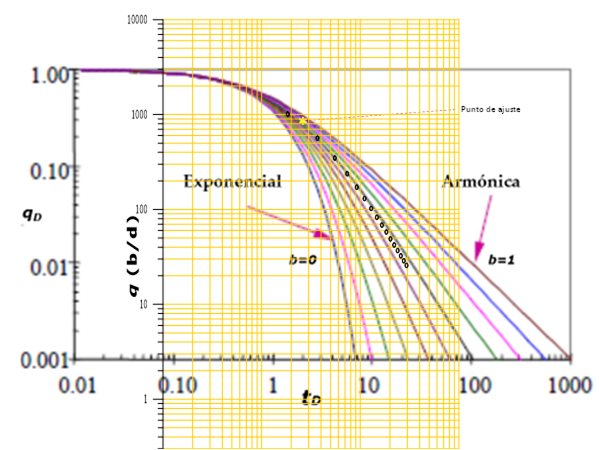
Where q is the mass flowrate in b/d, t is the time in months and b is the exponential constant for declining of Arps (1945) and Fetkovich (1980) equations. Figure 1 shows the type curve (Fetkovich, 1980), obtained through the Arps (1956) equations system.
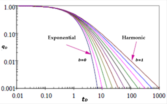
By considering equation (3), for b = 0 (n = 0, in Figure 1) the decline is exponential type. For b = 1 (n = 1, in Figure 1) decline is harmonic type. Both types of declining are the limits of the type curve while for the cases in which 0 < b < 1 the decline is hyperbolic type.
In the other hand, the equation to determine the cumulative production (Np) in barrels is as follows (Arps, 1956):
The variables in equation (4) are those as earlier defined. It is also possible to give the equation through a straight line by plotting log mass flow rate versus cumulative produced mass flow rate. The declining during the transitory period depends mainly on the formation characteristics near the well. It is important to stress that the apparent ratio of the well (r wa ) is utilized to determine the formation properties. Besides, the declining type curves are suitable for wells with damage factor (s) either positive or negative. The expressions of dimensionless parameters which are used in the type curve for the declining analysis are as follows:
For the dimensionless mass flow rate:
Where:
dimensionless mass flowrate (that represents the set of values of the ordinate axis in the type curve) |
|
value of the volumetric flow at time ( |
Dimensionless time is expressed by:
Where:
By substituting the value of q D , obtained from equation (5), in equation (7), the permeability (k) is obtained:
Equations (8) and (10) are used to determine the reservoir properties as follows, permeability (k) and porosity (φ), from the dimensionless mass flowrate and the time, respectivelly:
However, due to the volcanic nature of the geothermal systems, it has not been clearly defined the reservoir thickness (h) while fluid viscosity (μ) varies according to boiling processes occurring at the reservoir, for this reason it is a common practice to determine the transmissivity (kh/μ):
By substituting the dimensionless time (t D in equation (6)), in equation (10), the porosity φ, from equation (11) can be obtained:
By multiplying both sides of equation (11) for the variable h, the terms are grouped as follows; on one part the transmissivity (kh/μ), given by equation (9) and on the other part the storage φc T h, which is the same term that the one used in discharge tests in hydraulic engineering:
The uncertainty around the variables h and μ, leads to determine a direct value for permeability k in equation (8) or indices related to other variables (kh; k/μ). In Table 1 the formation indices that can be determined as a function of the knowledge of these uncertain variables.
Table 1 Known values related with formation permeability which can be determined according to knowledge of h and μ variables, using dimensionless flow equation on the type curves.
| Thickness( |
Viscosity ( |
Determination | Name |
|---|---|---|---|
| Known value | Known value |
|
Permeability |
| Known value | Unknown value |
|
Mobility index |
| Unknown value | Known value |
|
Capacity index |
| Unknown value | Unknown value |
|
Transmissivity index |
The first analysis methods based on type curves were applied to reservoirs to analyze pressure tests (Agarwal, Alhussainy & Ramey 1970; Earlouger & Kersh, 1974). By using the same analogy, the Slider (1983) superposed method has a similar procedure that the (log-log) type curves fit which are used to analyze increase/decrease pressure data for constant mass flowrate.
A simplified approach to determine the water inflow in finite systems which has provided results that can be favorably compared to those obtained using more rigorous analytical solutions for constant pressure, is that proposed by Fetkovich (1973).
Where:
productivity index in |
It is:
where
Considering that for initial conditions there is no pressure drop, the productivity index at initial conditions is given by:
Substituting equation (16) in equation (15), as following:
Now, substituting equations (15) and (17) in equation (13), it follows:
Which can be considered as a derivative of the exponential declining equation in terms of reservoir variables for constant pressure.
It is suggested that at the initial step of a declining analysis a general diagnosis of the production history behavior should be made. In Figure 2 a typical production curve along with the wellhead pressure and discharge orifice diameter vs time is given (Aragón-Aguilar et al., 2013). The last section of the plot can be fitted to a mathematical form and then can be extrapolated to a future time, in such way, it is possible to predict the well production for example to 1, 2, 5, 10 or more years.
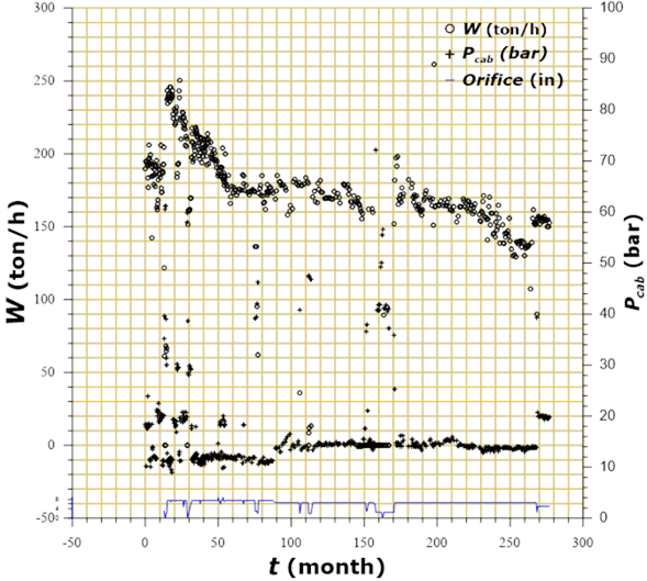
The production mass flow rate versus time plot allows to identify how the mass flowrate declines as a function of exploitation time. As an auxiliary plot, the one corresponding to the changes in discharge production orifices of the well over time is useful. By analyzing the variations in the orifice diameters and the behavior of production parameters (pressure and mass flowrate) it is easily seen how sensible they are and the close dependence existing between them. The case more noticeable is for the time interval of between 250 and 265 months, in which it is seen that the orifice diameter reduction has effect on both, the decrease in mass flowrate and the increase in pressure.
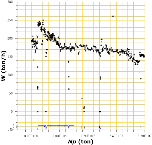
Furthermore, when plotting a graph with production data of a well vs the cumulative extracted mass production, it is observed that the part of the curve that declines can become a straight line, from which, extrapolations can be made, as shown in Figure 3. It is important to mention that in Figure 3 there appear two evolution trends for declining, the transitory (in the initial stage of exploitation) and the pseudo-steady state. As it is seen, when the slope of the curve changes in Figure 2, there is no orifice diameter variation, and hence, it is assumed that the change is due to the actual response of the reservoir.
Applications to practical field cases
In order to demonstrate the practical application of decline analysis theory, production data from an oil well, a geothermal and a water well were used. Below are the applications in these cases:
Petroleum well
An oil well produces in an area of low permeability, with a bottom pressure flowing of 800 lb/(in 2 ) abs (55.15 Bar). Measured data for the decline in the well discharge are listed in Table 2. Meanwhile Table 3 shows well data and results of a pressure increase test.
Tabla 2 Flow rate decline of a well at a constant
|
|
|
|
|---|---|---|
| 6 | 619.3 | 4 102.8 |
| 18 | 512.9 | 3 397.9 |
| 28.8 | 436.4 | 2 891.2 |
| 42 | 381.4 | 2 526.8 |
| 52.8 | 331.5 | 2 196.2 |
| 66 | 264.4 | 1 751.7 |
| 75.6 | 250.6 | 1 660.2 |
| 90 | 234.9 | 1 556.2 |
| 102 | 234.9 | 1 556.2 |
| 114 | 189.4 | 1 254.8 |
| 126 | 170.0 | 1 126.2 |
| 138 | 152.7 | 1 011.6 |
| 150 | 137.1 | 908.3 |
Tabl3 3 Characteristic data of rock formation at the wellbore.
| Parameters | Value | Unit |
|---|---|---|
|
|
1.36 | |
|
|
1.09E-6 | 1/(lb/in2)abs |
|
|
0.392 | mD |
|
|
121 | Foot |
|
|
5790 | (lb/in2)abs |
|
|
800 | (lb/in2)abs |
|
|
0.25 | Foot |
|
|
1490 | Foot (160 acres of spacing) |
|
|
-3.85 | at r wa = 11.75 |
|
|
0.101 | |
|
|
0.46 | cp |
In a complete well production study, the following characteristics are determined:
The production decline model in the well extrapolating it to the point where the flow reaches 10 (b/day) (approximately 66.25 lt/h), as critical limit.
Using declination data, q i and D are calculated. Subsequently, using Arps (1945) decline equation, q i is determined.
Calculated values of q i and D of point 2 are compared with the values determined with equations (1) and (2) using results of a pressure increase test.
Initially, in order to have a complete characterization of the test, a flow rate as a function of time graph is useful (Figure 4), which can be used as an auxiliary for the general diagnosis. After doing a general conceptualization of the test, the flow declination model is identified, for which two graphic methods are used:
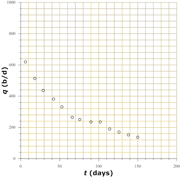
Figure 5 shows the log-log graph of
production data as a function of time, which is useful for acquiring a
previous idea of declination behavior. Figure
6 is a graph of the flow logarithm as a function of time,
elaborated using data in Table 2.
Through data adjustment, the equation of a straight line corresponding to
equation (3) (
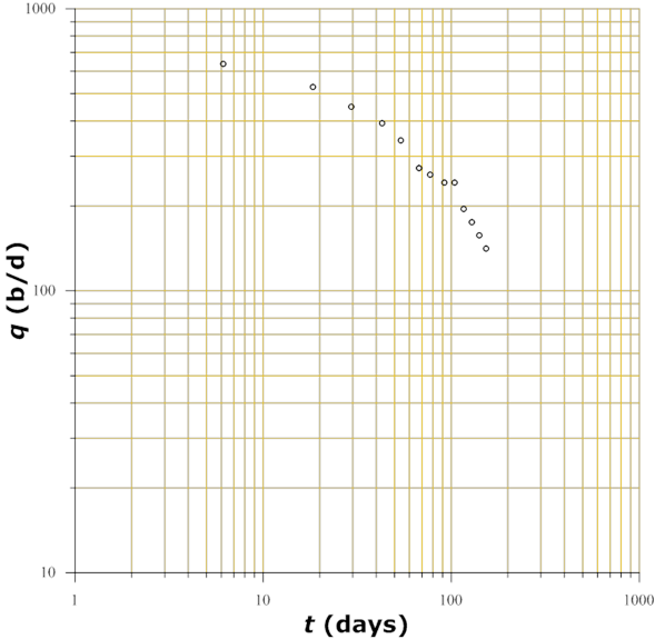
Figure 5 Log-log graphic of flow rate versus time, using data of the analyzed well (Golan & Whitson, 2003).
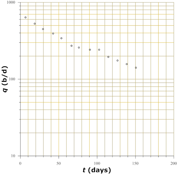
Figure 6 Graphic showing flow rate in logarithmic scale versus times, whose data corresponds to the analyzed well and are shown in Table 2 (Golan & Whitson, 2003).
The adjustment to a straight line allows us to obtain its characteristic parameters (the ordinate to the origin and its slope). The ordinate to the origin corresponds to the initial flow q i , while with the slope the decline rhythm (D) is obtained. In this way the values are:
In the absence of historical production measurements, parameters of equation (3) can also be determined from reservoir data. With equations (1) and (2), q i and D are determined using data obtained from transient pressure tests. Table 3 shows the values determined from a pressure test carried out in the well.
Applying equation (1) and replacing pressure test values, we get:
Applying equation (2) and substituting the values provided in Table 3, we obtained:
Values of q i and D calculated with Arps equation (1945), differ slightly from values obtained using the equations proposed by Fetkovich. This is due to particular considerations with which both methods were developed, however what should be highlighted from the methodology is that it provides a criterion on the range of the parameters of the decline in the analyzed well. Likewise, the high value in the well decline rate can be identified in conjunction with its low initial flow rate. Due to previous reason to illustrate the use of type curves, Table 4 shows time data, volumetric flow and accumulated production of another oil well, with which an analysis of the decline of its production is developed.
Table 4 Measured data: time (
|
|
|
|
|
|
|---|---|---|---|---|
| 180 | 940.00 | 169 200 | 6 227.50 | 26.902 |
| 360 | 522.67 | 263 280 | 3 462.69 | 41.861 |
| 540 | 323.33 | 321 480 | 2 142.06 | 51.115 |
| 720 | 221.17 | 361 290 | 1 465.25 | 57.445 |
| 900 | 159.17 | 389 940 | 1 054.50 | 62.001 |
| 1 080 | 120.93 | 411 708 | 801.16 | 65.461 |
| 1 260 | 95.00 | 428 808 | 629.38 | 68.180 |
| 1 440 | 76.67 | 442 608 | 507.94 | 70.374 |
| 1 620 | 63.50 | 454 038 | 420.69 | 71.192 |
| 1 800 | 53.67 | 463 698 | 355.56 | 73.727 |
| 1 980 | 45.50 | 471 888 | 301.44 | 75.030 |
| 2 160 | 39.23 | 478 950 | 259.90 | 76.153 |
| 2 340 | 34.23 | 485 112 | 226.77 | 77.132 |
| 2 520 | 30.13 | 490 536 | 199.61 | 77.995 |
| 2 700 | 26.73 | 495 348 | 177.09 | 78.760 |
| 2 880 | 23.90 | 499 650 | 158.34 | 79.444 |
In order to have a general diagnosis for the well behavior analysis, with the data provided, the graph of Figure 7 is developed, which illustrates the behavior of the flow with respect to time in Cartesian coordinates. Figure 8 shows the graph of the same variables in double logarithmic coordinates.
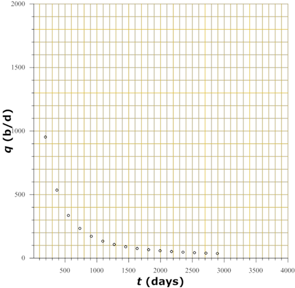
Figure 7 Data production behavior as time function in order to carry out a general diagnosis on the parameters behavior.
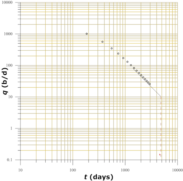
Figure 9 shows the behavior of the volumetric flow (q) with respect to the cumulative produced volume (Np). Figure 10 shows the overlap of production values (time, flow rate) on a double logarithmic scale on the type curve of Figure 1. It is convenient to emphasize the special care that must be taken in that the scales of both graphs are of the same magnitude to identify the type curve that best fits with the measured data.
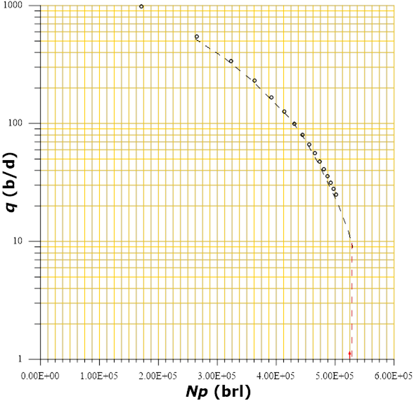
Figure 9 Graph showing volumetric flow rate (
Using the graph in Figure 8, and the production data in Table 4, it is assumed that the well has declined approximately 97.5% in 2 880 days. From the graph it can be inferred that at this rate of decline the critical flow limit (10 t/h) would be reached approximately a little less than 5 000 days. When using the analytical method, values closest to the extrapolation are selected from the well production history and are adjusted to an equation whose resulting expression is:
The combination of the accumulated produced volume (Np) and the volumetric flow (q) is used to determine the maximum recoverable volume in the well, that is, the total reserve. Assuming an output of 10 b/d as the economic limit of the well, the maximum producible volume can be determined by extrapolating the graph to this limit value, as shown in Figure 9. The graphical determination for this case turns out to be slightly higher than 500(103) b, which, could be assumed as the total reserve of the well. The adjustment equation obtained for this well is given by:
Data in Table 4 show that the cumulative production in the well is 499 650 (b), this value represents 97.8% depletion in the reserve, therefore the remaining reserve is 2.2%. However, the approximate time in which the economic limit of the well will be reached is 4 854 days. That is, the 2 880 days that the well has been producing represent 59.3% of the total estimated useful life. It would seem that it is an excellent well, because it still has a 40.7% useful life. However, it must be considered that the initial flow rate in the well is 940 (b/d) and at 2 880 days the flow is 23.9 (b/d). This means that the accumulated produced mass represents 97.9% of the total exploitable fluid. Therefore, in the last 1 974 days of useful life (4 854 - 2 880), the remaining reserve of 10 750 (b) (510 400 - 499 650) will be extracted at a flow lower than 23.9 (b/d), until reaching to the economic limit.
As can be seen in Figure 10, the flow as a function of time data plotted on log-log paper fits the standard curve whose value of n equals 0.5. According to the adjustment of production data of the analyzed well, it can be inferred that its type of decline is hyperbolic.
Values of the set point resulting from the comparison between the values plotted (t, q) in log-log scale and the type curve of Figure 1 are:
For the graph of measured values in the well, we have: t = 180 and q = 1000.
While the values corresponding to the same point in the type curve are: (t D ) = 1.4 y; (q D ) = 0.38.
The determination of the initial volumetric flow (q i ) and the initial declination rate (D i ) are obtained by means of the substitution of the previous values in equations (5) and (6), as shown below:
and
Furthermore, from the values of the dimensionless variables t D and q D , obtained in the adjustment with the type curve, it is possible to determine the characteristics of the formation by applying equations (8) and (11). To satisfy the conditions of the reservoir variables that these equations require, values obtained through the use of other techniques are used, such as pressure tests, laboratory measurements and/or geological or geophysical studies.
With equation (8) is obtained, according to Table 1, the permeability (k) or depending on the variables (kh) or (k/() is obtained or (kh/() of the formation with the equation (9). Whereas with equation (11) the porosity ( is determined, or in its case the storage of the formation (C T h with equation (12). This depends on the knowledge of the thickness of the production formation (h), the viscosity of the fluid (() and the total compressibility of the system (C T ). The volume factor (B) is obtained from laboratory analysis on the behavior of the fluid starting from background conditions and ending in surface conditions. The initial pressure (p i ) is determined from the measurements doing in the well. It is possible to determine the background pressure flowing (p wf ) either with the transient pressure tests, or through the use of simulators or, if possible, also from measurements with recording tools.
Case of a geothermal well
Throughout the development of the geothermal industry many of the techniques applied to oil fields have been adapted for their application in geothermal systems. The only condition for the application of this methodology is to take into account the fluid characteristics of each system, maintain consistency in the units and be careful in the use of the corresponding conversion factors.
Ordinarily in geothermal wells the production is expressed in mass flow (W) unlike how it has been expressed for oil wells that the volumetric flow (q) is used. In order to demonstrate the use of decline analysis techniques, the graph of Figure 11 is shown, which corresponds to production data from a well of a Mexican geothermal field (Arellano, Torres & Barragán, 2005; Aragón-Aguilar et al., 2013). Well production history covers a period of 340 months and in this graph it is possible to observe the behavior of its mass flow, its head pressure and its discharge orifice diameters as a function of time.
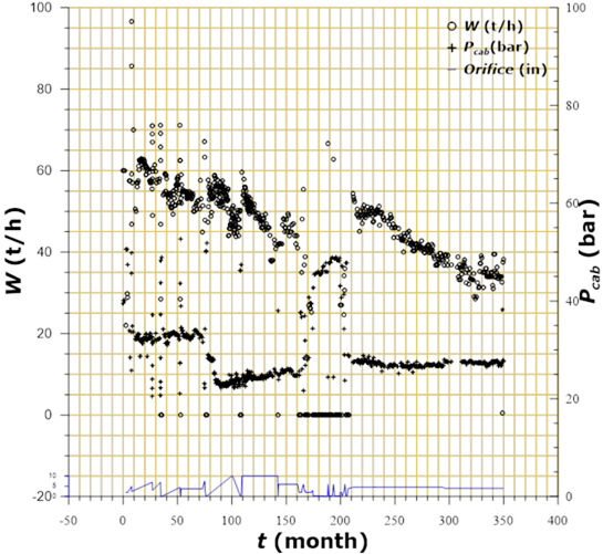
Figure 11 Plot for general diagnosis of behavior of well production its pressure at head conditions and variation of discharge orifice as function time.
The utility of the graph for the general diagnosis of the data and its application to the analysis of declination is oriented to obtain a vision of the general behavior of the test. As more data correlated with each other is available, an analysis with greater reliability can be doing. This is because in field operations it is not always possible to keep the flow constant, which influences the pressure.
Due to fluid mobility and boiling processes to maintain the discharge pressure in geothermal wells, variations in the orifice diameter are applied; however, the declining behavior in production prevails. One of the diagnostic plots is shown in Figure 11, in which the declination behavior in flow measurements can be identified under different opening conditions of the well discharge orifice.
In this figure it is possible to identify a closure in the well, in the period of time between months 150 and 200, which causes the head pressure to increase abruptly, reaching values close to its static condition. However, when opening the well again to a discharge hole similar to the one that was operating, the flow is slightly higher (by approximately 5%) than it existed at the time of closure. The above is evidence that the closure caused a slight recovery in the well, however the trend in the decline remained with a slope similar to the one that had been showing before the closure.
Figure 12 shows the graph of production data as a function of time. This same graph, but in log-log scale, is the one used within the adjustment methodology by comparison with the type curve.
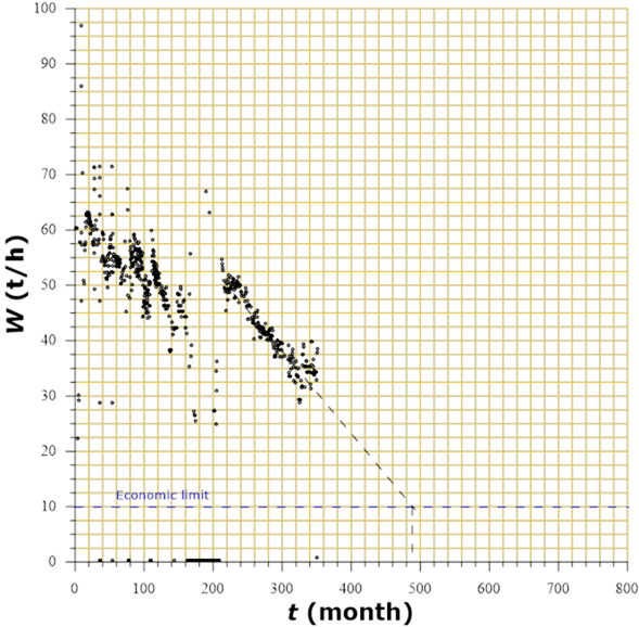
Another interesting application of this graph is its usefulness to determine the time in which the well, according to the trend in its decline, could reach the economic production limit. In the case of geothermal fields, the economic limit is governed by the plant capacity index to generate at least 1 MWe, with 10 (t/h) of steam at 7 bars of pressure. In accordance with the above, the graph shows the extrapolation of the last slope of the declination trend until the value for mass flow of 10 (t/h) is cut. Graphically, it can be seen that the time at which the flow reaches the economic limit is approximately 495 months. Using data adjustment of this last declination section with constant slope, an equation with the following form is obtained:
Being able to determine the value of t = 492 months, for W = 10 (t/h); which is a value close to that obtained graphically. According to the results obtained by one part, from graph 11 it is assumed that the well already has approximately 340 months of production. Therefore, the remaining time of production could be estimated at approximately 152 (492-340) months. That is, the well has already consumed, approximately (340/492), 69% of its productive life.
The declination constant of the well and the parameters of the formation are obtained through the graph of Figure 12, taking care that the logarithmic axes are of the same magnitude as those of the type curve. In order to obtain the parameters of the formation, this graph is compared with the type curve of Figure 1 and the curve to which the data fit best is searched. This procedure is shown in Figure 13.
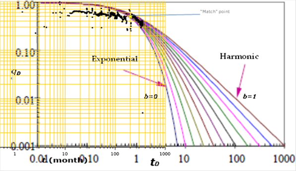
Figure 13 Overlapping of production data on the type curve for determining decline type through fitting technique.
Values of the match point that are determined in each graph are:
For the log-log graph (measured data): t=50 (months); q=50 (t/h)
While for the type curve, we have: t D =0.22; q D =0.78
The determination of the initial volumetric flow (q i ) and the initial decline rate (D i ) is carried out by means of the substitution of the previous values in equations (5) and (6). Therefore, we get:
And applying equation (6):
In relation to the initial expense (q i ) obtained from the type curve, it is convenient to mention the graphs of Figures 11 and 12. In both it can be seen that even when there is dispersion in the values, an initial value of the mass flow (q i ) can be estimated, close to 64 (t/h), which is congruent with that obtained using equation (5).
Using equation (7) a typical value of B was assumed for a geothermal system and a well flow simulator was used to determine (p i -p wf ). Special care was taken to use consistent units for the calculation of the transmissivity value of the formation:
On the other hand, using equation (8), and replacing the value of the transmissivity previously obtained, it is feasible to determine the storage of the formation. The apparent radius value r wa of the well is obtained from pressure tests. However, in the absence of more information, a range between 1E2 and 1E3 can be assumed, so values according to this variation are obtained. Substituting values and using consistent units we get:
Due to the uncertainty in the knowledge of r wa , the result can be left indicated as a function of this variable. From this point of view, the storage value for this well is equivalent to :
In oil reservoirs, the compressibility of the formation (C t ) and the thickness (h) are parameters that can be determined by measurements and for this reason the porosity value (() can be calculated directly. However, in geothermal systems, compressive experimental data are generally not available, due to the impossibility of preserving the reservoir temperature in the core test, in their transfer to laboratories. Likewise, it is not possible to determine with certainty the thickness (h), because most of the geothermal systems are nested in volcanic formations, whose characteristics cause uncertainty in the determination of the length of the production thicknesses. Therefore, it is an ordinary practice in geothermal systems to determine an index of transmissivity (kh/() and the storage (C t h instead of the permeability and porosity that is calculated in oil systems.
The other graph that is used is the flow against cumulative production (Np), whose extrapolation to the economic limit allows the estimation of the total reserve of the well, as shown in Figure 14. The behavior of production, closer to the extrapolation is considered representative by the overcoming of the transitory effects in the analyzed well. For this reason, the last slope of the declination trend was selected, extrapolating it to the economic limit of the flow of 10 (t/h).
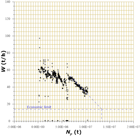
Figure 14 Behavior of cumulative produced volume as function of mas flow rate, for determining the feasible reserve.
With the graphic interpolation it is obtained that when reaching the economic limit, the cumulative produced fluid (Np) would be 14.75 E6 (ton), as can be seen in Figure 14. By adjusting the data of this last period an equation is obtained as follows:
Writing the expression to obtain Np as a function of W, we obtain :
Substituting the value of W = 10 in the previous expression, we obtain the value of Np=14.794 (106 (ton)), which represents the total reserve of the well. According to the measured data, the accumulated produced mass in the analyzed well is a little more than 10x106 (ton), which represents an approximate recovery of 67.6% (10/14.794) of the total reserve.
Case of a water well
Data used in this work correspond to water well located in the zone of
Oakwood of Montogomery, Ohio, USA (Dursch
& Wenclewicz, 2017). The well is completed in a thickness
with high hardness water (
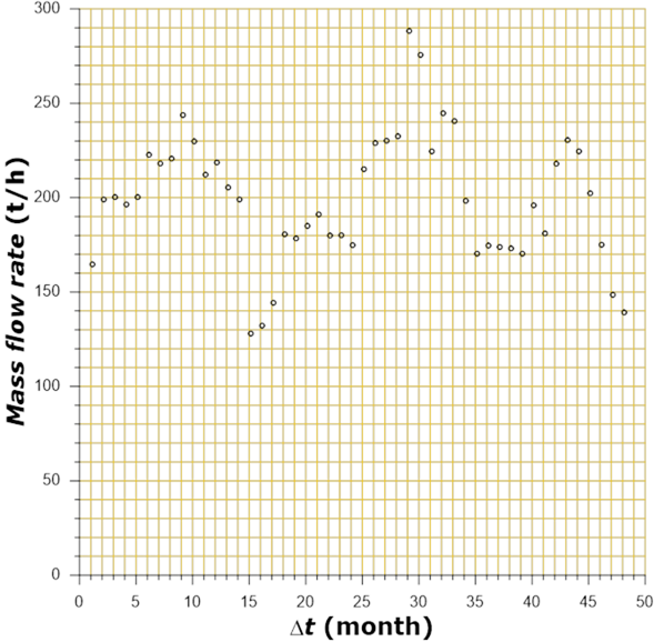
Figure 15 General diagnosis graph, showing behavior of water well productivity (Dursch & Wenclewicz, 2017), as exploitation time function.
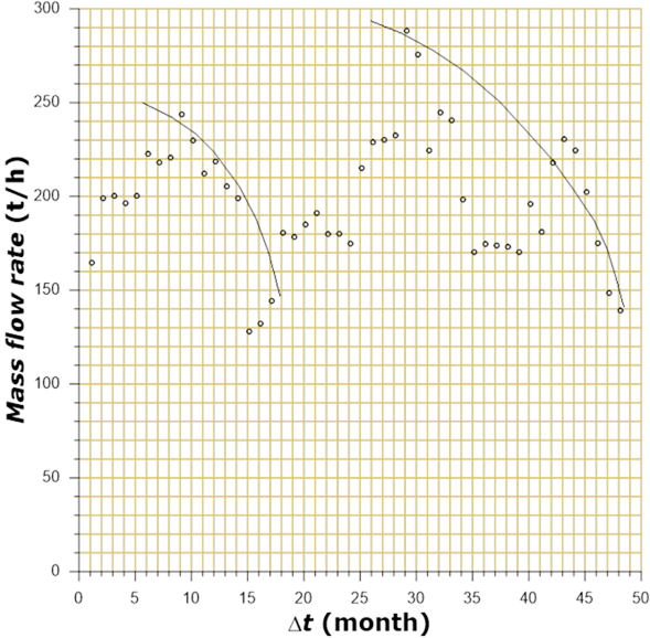
Figure 16 Productivity behavior of water well (Dursch & Wenclewicz, 2017), showing two decline periods: the first at early time (between 9 and 16 months) and the second, since the month 28 of its productive life.
Using the well data, is carry out a graph of log (flow rate) versus time as
shown in Figure 17. A data fit to a
line according to equation
(3)
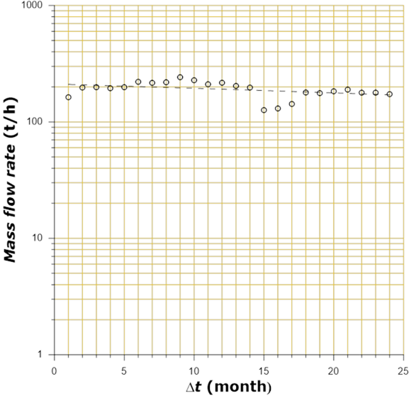
Figure 17 Graph of flow rate logarithmic versus time for determining the initial water flow rate (Dursch & Wenclewicz, 2017) using fit to a line.
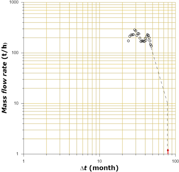
Figure 18 Log-log graph (flow rate versus time) using the more recent production decline data of the water analyzed well (Dursch & Wenclewicz, 2017), after established an economic productive limit.
After had been established an economic productive limit of the well in10 (t/h) and using log-log methodology of cumulative produced mass (Np) as flow rate (q), function, the total extractable of the well is determined, as shown in Figure 19. Knowing the difference between cumulative produced mass, the maximum reserve, the useful life and economic limit, remaining reserve is determined, which in this case results in 264 MM (ton).
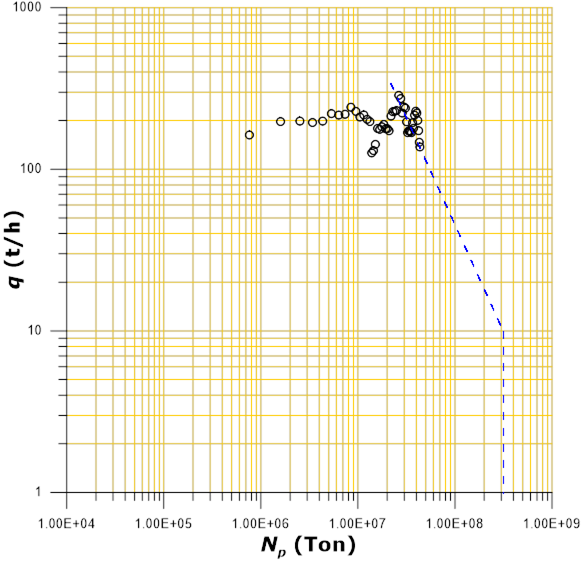
Figure 19 Produced mass (
After the first production decline in the well, jobs for improving its productivity were carried out (Dursch & Wenclewicz, 2017) it, resulted in an production increase. However, a year later, the well again showed decline tendency (month 28). Under such circumstances, in this work, in Figure 20 and Figure 21, two analyzes using the type curves technique are shown.
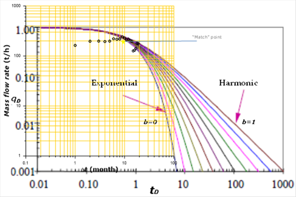
Figure 20 Measured production data, in water well, at early time period, graphed on the decline type curve proposed by Fetkovich, (1973).
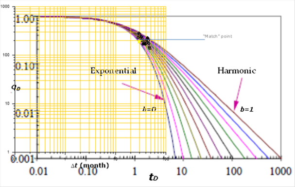
Figure 21 Measured production data, in water well, at late period, graphed on the decline type curve proposed by Fetkovich, (1973).
Figure 20 shows the fit with the type-curve, using data of the first decline trend. While Figure 21 shows the fit with the type-curve, using data of decline trend, from month 28 of operative well life.
According to the fit with the type-curve for the first period it can be determined a decline trend of “harmonic” type. This behavior is related with productive characteristics of the well taking into account its storage and feed.
For decline analysis in the first stage, through the use of data on the type curve and taking care for achieving the best match, following values are obtained :
For log-log graphic (measured data):
While, for the type-curve, are obtained
Determination of initial volumetric flow rate (
In relation with initial flow (
For period time of major system depletion, wich in this case is associated
with decline trend of the second stage, match point of the well data on the
type-curve, show different behavior. The achieved fit by comparing measured
data with the type-curve, shows a decline of "Hyperbolic" type,
with coefficient
For decline analysis at second stage, data of the well are graphed on the type-curve, treating to obtain the best match. In this case, it were obtained the “match” point values determined for each graph, as following:
For the log-log graph (measured data):
While for the type-curve are obtained
The initial volumetric flow rate determination (
In relation with initial flow (
Results of the developed analyzes have their practical application in obtaining technical criteria for the formulation of well exploitation designs and their future management. Table 5 shows a summary of results of the main parameters that support the arguments for decision making. Special care was taken to show the results of the analysis of the well data used in the examples with their respective work units. Each column of the table explains itself and shows the parameters with which it is feasible to configure decisions related to wells management.
Table 5 Summary of obtained results from production decline analysis
which are useful in individual characterization of well. Where,
| Type of well | Initial flow rate |
|
Total reserve | Total useful life | Remaining reserve |
|---|---|---|---|---|---|
| Petroleum well |
|
|
|
months | |
| 2 631 | 0.24 | 510 400 | 161.8 | 10 750 |
|
| Geothermal well |
|
|
106(ton) | (months) | 106(ton) |
| 64 | 0.0044 | 14.8 | 492 | 4.794 | |
| Water well |
|
|
106(ton) | (months) | 106(ton) |
| 211 | 0.053 | 310 | 78 | 264 | |
Within results of decline analysis that have been exposed it is advisable to involve the petrophysical characteristics of the formation (kh/() and ((C t h), to achieve an integral characterization of the well. In this research we have reviewed two analysis techniques: The type curves and the decline analysis and its application to petroleum and geothermal systems. The application of the analysis methods to hydraulic systems would not represent complications since it is a fluid in a single phase.
Discussion
Equations adaptation of petroleum systems to geothermal and hydraulic systems allows to reach reliable results. Only, it is necessary to be careful in the consistent handling of the work units. In the behavior shown in Figures 2 and 3, it can be assumed that there is a direct response from the reservoir. This is due to the fact that changes in the slopes of the graphs occur independently of the manipulations in the diameters of production holes.
It can be seen that in the initial flows (q i , W i ) there is congruence between measured and determined values, using the method of the type curve and equation (6), which supports the certainty of the methodology. Determinations were doing in wells with different fluid characteristics, so even though the methodology was developed for oil wells, with the results obtained, it is feasible to apply it to geothermal wells.
The geothermal well was closed for an approximate period of 50 months, identifying that the transitory effects are overcome and its pseudo-stable conditions are obtained even after approximately 150 months of continuous operation. This behavior is characteristic of systems where there is a recharge input. In geothermal systems the source of heat is constant; therefore, the water inlet represents the recharge. Therefore, farm design is based on the balance between the heat supply, the water inlet and the mass flow extraction.
Majority of geothermal systems are open aquifers, so there is a recharge water inlet that influences the presence of storage effects, which are manifested mainly under static conditions in the well. The graph of Figure 11 identifies the effects of storage at the opening of the geothermal well after a closure period. That is, when opening the well again it is observed that flow conditions are slightly higher than those that were before the closure, however when opening the well again the decline results with the same decreasing slope. The conjunction of the recharge water inlet and the heat supply are the basic characteristics to consider geothermal systems as renewable energy. A hydraulic system is considered renewable when being fed by a water entrance.
Through the different stages of the production behavior, the well first shows the transitory effects and then the pseudo-stable state. Data used correspond to their pseudo-stable conditions, useful for obtaining their equations and their extrapolation towards decline future trends. The value of 10 (t/h) of flow, assumed as the economic limit for a geothermal well, still represents a lot of energy that can be applied in other forms of exploitation. The important aspect about the methodology is the determination of the total and remaining reserve, regardless of the economic limit established.
The useful life of a well is linked to its reserve and recharge. The advantage of geothermal and hydraulic deposits over oil deposits is that the water inlet provides recharge that adds to the system's own storage. For this reason, decline rates of these are lower compared to those of oil fields. This same recharge factor influences the lifetimes of each system. In oil deposits the initial volume is no longer modified over time, because there is no generation of new hydrocarbons.
Behavior of water well productivity indicates a tendency to decline due to effects provoked by high salts content obstructing flow channels. By this reason, it is explainable that after be repaired, firstly presented a recovery in its production, however, after a brief operation time again the well adopted the decline tendency.
Conclusions
The production decline analysis is a useful technical tool for aquifers and petroleum and geothermal reservoirs characterization.
From research carried out, it has been found that influence parameters in production decline of analyzed systems, are formation properties, storage, flow rate and recharge.
The advantage of geothermal and hydraulic systems over those of petroleum is the water entrance which represents the substantial recharge, influencing in diminish of decline rate and expanding the useful life and remaining reserve.
It is appropriate to highlight that tendency of decline is a single characteristic of each well. Even though could be interrupted by external factors such as cleaning, maintenance, temporal close, repairs, etc., however, when exploitation continues, decline maintains its trend.
In production decline analysis, it is important to identify, reservoir response, transient states, and pseudo steady state.
The properly correlation of mass flow rate, cumulative production and time is a useful technical base for prediction of future behavior, determination of economic useful life and remaining reserves.
By establishing economic production limits of each well, it can be determined, from its decrease trend, its economic useful life. It is important to identify the feasibility of the project as gets to economic limit.
Correlation of cumulative produced volumes, economic limits and decline tendencies allow determine maximum volumes can be produced.
Behavior characterization of each well and its correlation with production economic limits allow determine the maximum reserve could be recovered, influencing in exploitation planning.
Production decline analysis and its knowledge of future trends help to exploitation designs establishment and taking decisions about feasible jobs for its productivity enhance and field expansion planning.
Acknowledgements
Authors thank to Instituto Nacional de Electricidad y Energías Limpias (INEEL) by the support given for developing this work under project IIE-14454 “Técnicas y métodos de análisis, al estado del arte de declinación de la producción en sistemas geotérmicos mexicanos y sus efectos predictivos”.
REFERENCES
Agarwal, R. G., Al-Hussainy, R., & Ramey, H. J. Jr. (1970). An investigation of wellbore storage and skin effect in unsteady liquid flow: I. Analytical treatment. Society of Petroleum Engineers Journal, 10(03), 279-290. DOI: 10.2118/2466-PA [ Links ]
Agarwal, R. G., Gardner, D. C., Kleinsteiber, S. W., & Fussel, D. (1999). Analyzing well production data using combined type curve and decline curve analysis concepts. SPE Reservoir Evaluation & Engineering, 2(05), 478-486. DOI: 10.2118/57916-PA [ Links ]
Aragón-Aguilar, A., Barragán, R. R., Arellano, G. V. (2013). Methodologies for analysis of productivity decline: A review and application. Geothermics, 48, 69-79. DOI: 10.1016/j.geothermics.2013.04.002 [ Links ]
Arellano, G. V., Torres, M. A., & Barragán, R. M. (2005). Thermodynamic evolution of the Los Azufres México geothermal reservoir, from 1982 to 2002. Geothermics, 34(5), 592-616. DOI: 10.1016/j.geothermics.2005.06.002 [ Links ]
Arps, J. J. (1945). Analysis of decline curves. Transactions of the AIME, 160(01), 228-247. DOI: 10.2118/945228-G [ Links ]
Arps, J. J. (1956). Estimation of primary oil reserves. Petroleum Transactions, AIME, 207, 182-191. [ Links ]
Bahadori, A. (2012). Analysis gas well production data using a simplified decline curve analysis method. Chemical Engineering Research and Design, 90(4), 541-547. DOI: 10.1016/j.cherd.2011.08.014 [ Links ]
Blasingame, T. A., McCray, T. L., & Lee, W. J. (enero, 1991). Decline curve analysis for variable pressure drop/variable flow rate systems. En: Gas Technology Symposium, Society of Petroleum Engineers, Houston, Texas, 22-24 de enero. DOI: 10.2118/21513-MS [ Links ]
Cárcamo, T. E., & Polo, N. G. (2007). Metodología para la predicción de curvas de declinación de pozos de petróleo aplicando redes neuronales artificiales (tesis de licenciatura). Universidad Industrial de Santander, Santander, Colombia. [ Links ]
Dursch, G. L., & Wenclewicz, M. (2017). 2016 Water production annual report, City of Oakwood (pp. 14). Ohio, USA: Ohio Department of Natural Resources. [ Links ]
Earlouger, R. C., & Kersh, K. M. (1974). Analysis of short-time transient test data by type-curve matching. Journal of Petroleum Technology, 26(07), 793-800. DOI: 10.2118/4488-PA [ Links ]
Fetkovich, M. J. (1973). The isochronal testing of oil wells. SPE 4529 48 th Annual Technical. Conferencia llevada a cabo del 30 de Sept. al 3 de Oct, por la Society of Petroleum Engineers, Las Vegas, Nevada, USA. [ Links ]
Fetkovich, M. J. (1980). Decline curve analysis using type curves. Journal of Petroleum Technology, 32(06), 1065-1077. DOI: 10.2118/4629-PA [ Links ]
Fetkovich, M. J., Fetkovich, E. J., & Fetkovich, M. D. (1994). Useful concepts for decline forecasting reserve estimation and analysis. 60 th Annual Technical Conference SPE. Conferencia llevada a cabo por la Society of Petroleum Engineers, Nueva Orleans, Luisiana, USA. [ Links ]
Gaskari, R., Mohagheghi, S. D., & Jalali, J. (mayo, 2006). An integrated technique for production data analysis with application to mature fields. Gas Technology Symposium. Llevado a cabo del 15-17 de mayo por la Society of Petroleum Engineers, Calgary, Alberta, Canada. DOI: 10.2118/100562-MS [ Links ]
Golan, M., & Whitson, C. H. (2003). Well performance (2a ed.). Trondhiem, Noruega: Tapir Akademiske Forlag. [ Links ]
Gunn, C., & Freeston, D. (1991). An integrated steady-state wellbore simulation and analysis package. Proceedings of the 13th New Zealand Geothermal Workshop. Llevado a cabo por Geothermal Institute, The University of Auckland, New Zealand. [ Links ]
Mata, D., Gaskari, R., & Mohagheghi, S. D. (octubre, 2007). Field wide reservoir characterization based on a new technique of production data analysis: Verification under controlled environment. Eastern Regional Conference and Exhibition. Llevada a cabo el 17-19 de octubre por la Society of Petroleum Engineers, Lexington, Kentucky, USA. DOI: 10.2118/111205-MS [ Links ]
Sanyal, S. K., Menzies, A. J., Brown, P. J., Enedy, K. L., & Enedy, S. (1989). A systematic approach to decline curve analysis for the Geysers steam field, California. Geothermal Resources Council Transactions, 13, 415-421. [ Links ]
Shahamat, M. S, Hamdi, H., Mattar, L., & Aguilera, R. (2016). A novel method for performance analysis of compartmentalized reservoirs. Oil and Gas Science and Technology - Rev. IFP Energies Nouvelles, 71(3). DOI: 10.2516/ogst/2015016 [ Links ]
Slider, H. C. (1983). Worldwide practical petroleum reservoir engineering methods. Oklahoma, USA: Penn Well Books. [ Links ]
Received: August 03, 2015; Accepted: August 09, 2018
 Este es un artículo publicado en acceso abierto bajo una licencia
Creative Commons
Este es un artículo publicado en acceso abierto bajo una licencia
Creative Commons
