


 text new page (beta)
 English (pdf)
 Article in xml format
 Article references
 Send this article by e-mail
 Cited by SciELO
  Similars in
SciELO
Similars in
SciELO 
 Permalink
1. Introduction
Lean manufacturing is one of the initiatives that many major businesses have been trying to adapt to remain competitive in an increasingly global market. The focus of the approach is on cost reduction by eliminating non-value added activities (Abdulmalek & Rajgopal, 2007). These value-added activities make the final product or service more valuable to the end consumer(Hines & Rich, 1997). In general, the approaches aim to increase production efficiency (productivity) and quality and reduce work-in-progress, stock levels, and unnecessary product handling (Hicks, 2007).
The process of mapping the material and information flows of all components and sub-assemblies in a value stream that includes manufacturing, suppliers, and distribution to the customer is known as value stream mapping (VSM). Value stream map has proved effective in identifying and eliminating wastes in a facility with similar or identical product routings, such as in assembly facilities (Seth & Gupta, 2005).
Value Stream Mapping (VSM), a tool more focused on the entire value stream of a productive process. VSM is a mapping tool that is used to map a productive process or an entire supply-chain network (Braglia et al., 2006). Lean application is guided by 5 simple steps starting from identifying the value of process, identifying the process value stream, focusing on the process flow, configurations of the pull factor and work towards process perfection (Rahani & Al-Ashraf, 2012). The value stream mapping (VSM) method is used to explore the wastes, inefficiencies, non-valued added steps in a single, definable process out of the complete product development process (PDP) (Tyagi et al., 2015).
The tool value stream mapping (VSM) is applied as a way to progress toward lean manufacturing and as a formula to lead the activities of improvement. Kanban card has been used to identify problems of production flow, maintaining the synchronization of inventory and material flow among production cells (Alvarez et al., 2009). The goals of VSM are to observe material flow in real-time from the final customer to the raw material and to visualize losses in the process, using symbols to represent the process visually and clearly (Dal Forno et al., 2014). A lean approach stimulates a new direction of planning and performing activities effectively and efficiently in the manufacturing system (Grewal, 2008).
Value stream refers to those specifics of the firm that add value to the product or service under consideration. It usually starts with customer delivery and works its way back through the entire process documenting the process graphically and collecting data along the way (Singh & Sharma, 2009). By eliminating non-value added (NVA) factors and creating an overall smoother process, products and services become more valuable to the consumer as well as more competitive to rivals
on a market (Teichgräber & Bucourt, 2012). The utmost objective of lean production is to eliminate all activities that do not add value throughout the production process. Originally, it was designed to produce cars in Japan, but its main techniques have been applied to a wide variety of other processes in both services and manufacturing (Jiménez et al., 2012).
A value stream is a collection of all actions (both value-added and non-value added) that are required to bring a product or a product family that use the same resources through the main flows, starting with raw material and ending with the customer (Xia & Sun, 2013). In contrast to 4.0 lean production (LP) is based on standardized processes, finding abnormalities, problem-solving and continuous improvement to reduce waste activities and to achieve higher levels of flow. A short lead-time through a process chain (a value stream) results in a higher output therefore in higher productivity and thus increases the overall added value within this given period (Kuhlang et al., 2011; Meudt et a., 2017).
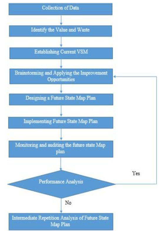
In this study current and future state map plan is generated for the company. Then there is the identification of improvement opportunities and accordingly action plan generated.
2. Materials and methods
2.1. Collection of data
The first step is the collection of data, see Figure 1. For applying the lean principle, the collection of data from the shop floor is much important. The data may include cycle time, uptime, downtime, TAKT time, material handling time, packaging time, and raw material arrival frequency. This data gives a rough idea about the current process and its efficiency. Collection of the shop floor data and software automation can easily allow you to make the process much efficient (Roser et al., 2014).
Data collection and its analysis offer help significantly to management for taking right strategic decisions.
2.2. Identification of value and waste
The activities that don’t contribute toward the product or process while the activities which add value to the product for which the customer is willing to pay.
There are several non-value added activities commonly found in the manufacturing sector:
- Process steps that are not needed
-Unnecessary movement of resources
-Rework due to defects in the product
-Corrections and rechecking
-Unnecessary storage of raw material more than required
-Waiting between workstations
Non-value-added activities directly affect processing or product cost. So identification and elimination of these activities are important.
2.3. Establishing current value stream map
Value stream map is the graphical representation of the entire organization’s processes in one map. It includes both material flow and information flow (Stadnicka & Litwin, 2017).
There is a time ladder at the bottom of the map which gives information about value-added and non-value::added activities so gives overall lead time in the entire process. By mapping a simple value stream map one can know about raw material quantity and its frequency, cycle time, uptime, downtime, lead time, actual processing time, outgoing finished goods quantity, and its frequency. The current value stream map gives improvement opportunities.
2.4. Design and implementation of future value stream map
The current state map gives an idea about the efficiency of the process line. According to setting the goal for the improvement which is an important part of the future state map. The future state map gives an idea about the efficiency of the processing line as compared to the current state value stream map (Esfandyari et al., 2011). Accordingly, an action plan should be generated. Then Implementation of the action plan and analysis of the results of plan is important.
2.5. Performance analysis and its repetition
After the implementation of the action plan, only performance analysis gives the results of the action plan whether the processing line is efficient or not. If results are positive then the future state map plan is considered as a current map and accordingly there is a plan for further improvement. If the results are negative then there is intermediate repetition is important till the outcomes are positive.
3. Experimental work
3.1. Production flow process
The processing line is of Axle Beam Housing. An axle is an actual crossbar supporting a vehicle, on which one or more wheel turn. Two wheels are connected by a shaft called an axle. It sits inside the Axle Housing and is held in place by bearings that allow it to rotate within axle housing.
Axle Beam Housing Material Specifications:
Material- SG450-10 (Ductile cast Iron).
Envelope Dimensions- 299.07 mm x 464.93 mm x 1549 mm
Final Mass in Kg- 189.204 kg
Tensile Strength- 450 Mpa
Yield Strength- 310 Mpa
Elongation- 10%
Hardness- 184 BH (Brinell hardness)
Chemical Composition- 3.44%, Si- 5.51%, Mn- 0.35 %, P- 0.04 %, Mg-0.02%
Weekly, 10 castings of housing arrived for machining at FIE, Ichalkaranji. The total processing of Axel Beam Housing is done in 5 stages, see Figure 2. The processing starts with a 100% inspection. The inspection is generally done with the help of the naked eye inspection. If any defects are detected, then the defective parts are transferred to the scrap house. From scrap house, they returned. Accepted parts are stored in the buffer for 1st stage machining of the casting. After processing in station 1 the castings should go through an inspection process where Surface Roughness, weight, and different holes are inspected using GO and NOGO gauges.
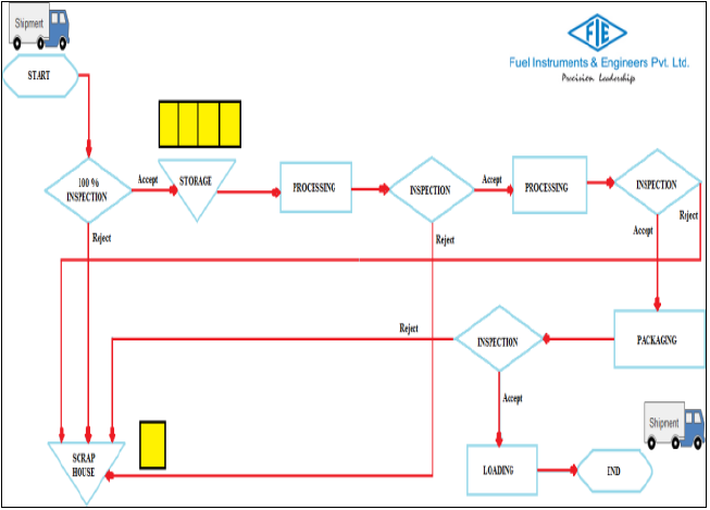
Rejected parts transferred to the scrap house. Accepted parts are transferred to station 3 for further processing. Again same process of inspection is done after machining at station 3. Accepted parts are transferred to the packaging. After packaging there is again inspection, this inspection is different in this case. Ok parts are dispatched for loading in the vehicle while rejected parts have resorted and again loading is done. Here the overall processing of the Axle Beam housing is done
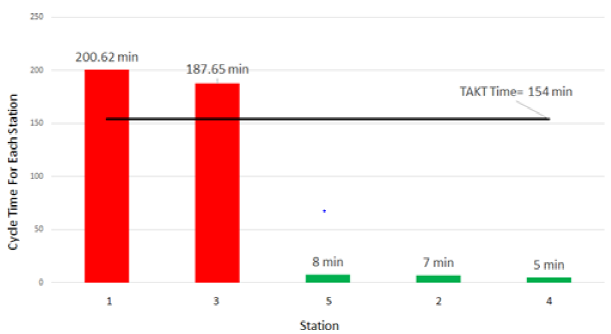
3.2. Cycle time and takt time calculation
The processing of the axle beam housing is done in 5 stations. Cycle time for these stations 200.62 minutes, 7 minutes, 187.65 minutes, 5 minutes, and 8 minutes.
TAKT time- It is the average time between the start of production of one unit and the start of production of the next unit (Figure 3).
No. of shifts per day= 2
8hr/shift= 8 x 60=480min/shift
Available time= 480 x 2= 960 min/day
Breaks= 30 min/shift
Start up meeting= 10 min/ shift
Lunch= 30 min/shift
End of shift clean up= 10 min/shift Machine
Setup time= 15min/shift
Customer demand= = 5 parts/day
TAKT time= Available time/day / Customer demand/ day
Actual Available time per shift 8hrs per shift= 480min/ shift
Total breaks per shift= 95 min
Total available time per shift= 480-95= 385 min/shift
Per day 2 shifts= 770 min/ day
Therefore,
TAKT time= 770 /5 = 154 min/part
To match customer demand the cycle time of the station should lie below than that of the TAKT time.
3.3. Control chart analysis
The final mass of the finished product should be 189.204 kg. The product weight is inspected for 30 days in a subgroup size of 2. Then the data is analyzed in the Minitab 19 software, see Figure 4.
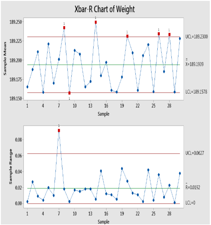
189.166, 189.164, 189.201, 189.174, 189.206, 189.215, 189.156, 189.160, 189.231, 189.211, 189.175, 189.165, 189.155, 189.247, 189.233, 189.251, 189.156, 189.158, 189.221, 189.204, 189.215, 189.200, 189.156, 189.174, 189.181, 189.163, 189.252, 189.247, 189.200, 189.159, 189.191, 189.203, 189.166, 189.155, 189.161, 189.156, 189.156, 189.200, 189.245, 189.217, 189.216, 189.203, 189.166, 189.155, 189.205, 189.207, 189.199, 189.241, 189.157, 189.161, 189.252, 189.216, 189.181, 189.189, 189.222, 189.245, 189.158, 189.159, 189.209, 189.247.
For Process, under control, all data points should lie within UCL and LCL values. For inspected data, the test failed at 8, 9, 14, 20, 26, 28. Hence, the process is not under control and needs corrective action. Basically, out of control process shows the presence of non-random variation. Non-random variation is caused by definite, specific causes that are called assignable causes. These assignable causes make the process go out of control. It is important to find the assignable causes and take action to remove them. Once assignable causes are removed the process will become stable and return to its controlled condition.
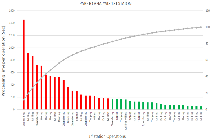
3.4. Cycle time and Pareto analysis chart
Pareto analysis is a technique in decision-making that is used for the selection of a limited number of factors that produce a significant overall effect. It states the 80% of problems arise as a result of 20% of causes. In this case cycle time for the operation is the factor that produces a significant impact on overall production.
The cycle time for each operation is calculated directly on the station 1 monitor reading. Readings are arranger in descending order. According to the Pareto principle, the first 20 operations are taken into consideration because the first 20 operations contribute much time in overall cycle time. The total cycle time for station 1 is 200.62 min (Figure 5).
The cycle time for each operation is calculated directly on the station 3 monitor reading. Readings are arranger in descending order. According to the Pareto principle, the first 19 operations are taken into consideration because the first 19 operations contribute much time in overall cycle time. The total cycle time for station 3 is 187.65 min, see Figure 6.
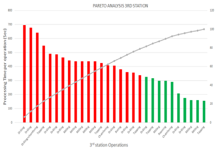
The main approach toward reduction for these factors. If these factors are tackled then the organization can drastically impact on 80% of problems. The cycle time of station 1 and station 3 is greater than that of the takt time of 154 min/part. Hence, station 1 and station 3 were taken into consideration.
3.5. Current value stream mapping
Current value stream mapping means it is the graphical representation of all entire processes of the organization on one paper (Kasava et al., 2015). The upper parts represent the Supplier, customer, and Production control department of the organization. While the lower part of CVSM is the time ladder which consists of value-added and non-value-added part. The upper part of the time ladder diagram represents non-value added activities and the lower part of the time ladder diagram represents value-added activities. The time on the ladder diagram represents the time required for the respective operation (Rother & Shook, 2003).
The orange bursts represent ”Kaizen” i.e. it shows improvement opportunities. The maroon triangle represents inventory between the station. The non-value added time can be calculated by taking a ratio of Inventory count to customer demand at each station. The lower right part of the paper represents overall time i.e., lead time (Figure 7).
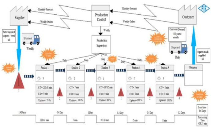
In this case, supplier and customer are the same. Customer sends monthly forecast and weekly orders to production control department via Email at FIE. Then production control sends weekly orders to the supplier. The supplier sends 10 parts per week. These 10 parts are stored at the initial stage of the processing line which uncontrolled inventory. In this case, the uncontrolled inventory count of part is 7. Then the parts are transferred to station 1 with a cycle time of 200.62 min and having an uptime of 70 %. 2 Station is an inspection station having a cycle time of 7 minutes and an uptime of 100%. 3rd station is a processing station with having a cycle time of 187.68 min. Station 4 and 5 are inspection and packaging stations having a cycle time of 5 and 8 min respectively
The timeline is shown at the lower part of the map, which shows value added time and non-value added time. The total lead time is 4.6 days and the total processing time is 408.27 min. The inventory count divided by customer demand gives lead time between stations. According to this process FIE able to ship 6-8 parts per week.
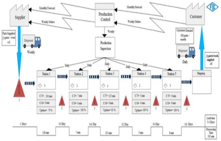
3.6. Future value stream mapping
In this case, supplier and customer are the same. Customer sends monthly forecast and weekly orders to production control department via Email at FIE. Then production control sends weekly orders to the supplier. The supplier sends 25 parts per week. These 10 parts are stored at the initial stage of the processing line which uncontrolled inventory. In this case, the controlled inventory count of part is 5. Then the parts are transferred to station 1 of cycle time 130 min and having an uptime of 70 and 5 are inspection and packaging stations having a cycle time of 5 and 8 min respectively.
The timeline is shown at the lower part of the map, which shows value added time and non-value added time. The total lead time is will be 3.4 days and the total processing time 245 min. The inventory count divided by customer demand gives lead time between stations. According to this process, FIE will able to ship 20 parts per week, see Figure 8.
Accordingly, the action plan generated for improvement and previously those cutters which contribute more cycle time in overall production are changed to new cutters which are much efficient as compared to previous. The new cutters are selected from different tool catalogs. For the cutters who have the ability but not set at its optimum level, their speed, feed, and depth of cut are set at their optimum level so that the required cycle time will be less and hence productivity will be higher.
3.7. Productivity calculations before implementation
Station 1:-
Cycle Time= 200.62 min
Up Time= 70%, Actual Processing Time= 539 min
Units produced per day= 2.688
Machining hrs per day= 12.833 hrs
Productivity= Units produced per day / Machining hours per day
Productivity= 2.688 units/day / 12.833 hrs/day
Productivity= 0.2094 Units/hr
Station 2:-
Daily Machining time Available= 770 min (2 shifts/day) Cycle Time= 7 min.
Up Time= 100%, % idle= 97.3 %, Actual Processing Time=770-749.21=20.79 min. Units produced per day= 2.97
Machining hrs per day= 12.833 hrs.
Productivity= Units produced per day / Machining hours per day Productivity= 2.97 units/day / 12.833 hrs/day
Productivity= 0.2314 Units/hr
Station 3:-
Daily Machining time Available= 770 min (2 shifts/day) Cycle Time= 187.65 min.
Up Time= 83%, % idle= 30.3 %, Actual Processing Time= 445.45 min Units produced per day= 2.37
Machining hrs per day= 12.833 hrs.
Productivity= Units produced per day / Machining hours per day Productivity= 2.37 units/day / 12.833 hrs/day
Productivity= 0.184 Units/hr
Station 4:-
Daily Machining time Available= 770 min (2 shifts/day) Cycle Time= 5 min
Up Time= 100%, % idle= 98.7 %, Actual Processing Time=770-759.99=10.01 min Units produced per day= 1.25
Machining hrs per day= 12.833 hrs
Productivity= Units produced per day / Machining hours per day Productivity= 2 units/day / 12.833 hrs/day
Productivity= 0.155 Units/hr
Station 5:-
Daily Machining time Available= 770 min (2 shifts/day) Cycle Time= 8 min
Up Time= 100%, % idle= 98 %, Actual Processing Time=770-754.6=15.4 min Units produced per day= 1.925
Machining hrs per day= 12.833 hrs
Productivity= Units produced per day / Machining hours per day Productivity= 1.925 units/day / 12.833 hrs/day
Productivity= 0.15 Units/hr
4. Results
This study has shown the implementation of a value stream map in axle beam housing processing line to reveal obvious and hidden waste that affected productivity.
The tool technology was implemented at station 1 and station 3 which have a cycle time larger than that of takt time. This technique was successfully implemented because cycle time in station 1 and station 3 was reduced from 200.67 minutes to 120.14 minutes and 187.65 minutes to 111.75 minutes respectively. VSM technology the current map plan is simulated in the Flexsim 2019 simulation software.
Then results of the simulation software were used for an action plan for further improvement. The main aim was to reduce the cycle time of station 1 and station 2 below 154 min. Then accordingly future state VSM was generated.
In the future state value stream map, the target for station 1 and station 2 was 130 min and 115 min. In the initial stage, there was a study of various cutters and their cutting ability from the respective tool catalog. The cycle time for each operation is calculated and a respective Pareto chart was developed. Only cutters were selected who contribute more cycle.
Some important results:
The cycle time of station 1 is reduced from 200.67 min to 121.33 min.
Units produced per day on station increased from 2.688 to 4.44.
Productivity increased on station 1 from 0.2094 units/hr to 0.3459 units/hr.
Units produced per day on station 2 increased from 2.97 to 6.05
Productivity increased on station 2 from 0.2314 units/hr to 0.4714 units/hr.
The cycle time of station 3 is reduced from 187.65 min to 111.75 min.
Units produced per day on station 3 increased from 2.37 to 4.409.
Productivity increased on station 3 from 0.184 units/hr to 0.3435 units/hr.
Units produced per day on station 4 increased from 1.25 to 4.928.
Productivity increased on station 4 from 0.115 units/hr to 0.3840 units/hr.
Units produced per day on station 5 increased from 1.925 to 5.005.
Productivity increased on station 5 from 0.15 units/hr to 0.39 units/hr.
5. Conclusions
The value stream map was introduced in this project work with a step-by-step guidance through the method. A practical example of a company shows how waste in informational logistics was eliminated so that the company could reduce the lead time from 4.6 days to 3.3 days. Previously, Fuel Instruments & Engineers could make 1 or hardly 2 parts/day. Currently, because of improvement in the organization, it can make 5 parts/day. In future research, a more detailed design of the individual steps will be developed. For example, relevant methods and tools in the different phases of the value stream map must be analyzed. Additionally, the method should be applied to other companies and branches.

