text new page (beta)
 English (pdf)
 Article in xml format
 Article references
 Send this article by e-mail
 Cited by SciELO
  Similars in
SciELO
Similars in
SciELO 
 Permalink
1. Introduction
Information on the current state of the economy is a crucial aspect in decision making for policymakers. Nonetheless, key statistics on the evolution of the economy are available only with a certain delay, which is why we rely on forecasting procedures in order to get timely estimations of those key figures. This is the case of series that are calculated on a quarterly basis, such as the Gross Domestic Product (GDP). Indeed, it is of a particular importance for central banks to use precise short-term GDP estimates in guiding monetary policies that will affect the long run; in the words of Lucas (1976:22), “...forecasting accuracy in the short-run implies reliability of long-term policy...”
Indeed, an increasingly common forecasting practice among central banks is nowcasting, which has been broadly studied in developed countries, such as China, France, Germany, Ireland, New Zealand, Norway, Spain, Switzerland, UK, United States (US), among others (and whose practice is much less generalized in developing economies, where it is mainly used by the IMF) with the purpose of obtaining timely GDP estimations. In particular, Mexico’s National Institute of Statistics (INEGI) publishes its estimate of Mexico’s GDP and the official measure of National Accounts four and seven weeks after the end of the reference quarter, respectively. And although forecasts from Bloomberg and from Banco de México’s Survey of Professional Forecasters (SPF) are updated on a regular basis, a more precise estimate of GDP would be helpful for policymakers.
For example, during the third quarter of 2019 (July-September), policymakers would prefer to take decisions based on that quarter’s data and on the short-term forecasts of economic activity. However, in Mexico, the firstGDP estimated figures were not released until October 2019, which means that policymakers had to wait about 120 days for needed GDP data and at least 30 days after the end of the quarter, in order to have the first reliable estimate of economic activity for that quarter (the rapid GDP estimate is conducted by INEGI). Furthermore, official GDP statistics for the third quarter are not published until the end of November, which means a larger delay in their availability and, hence, reducing its usefulness for decision making purposes.
My goal in this paper is to find a nowcasting model that is more accurate than the consensus GDP estimates of professional forecasters and the GDP estimations released by INEGI. I propose five nowcasting models that forecast quarterly GDP using monthly data (which are inspired by the work of Rnstler and Sédillot, 2003; Baffigi, Golinelli, and Parigi, 2004; Giannone, Reichlin and Small, 2008). These include a dynamic factor model (DFM), two bridge equation (BE) models and two principal components (PCA) models, which are the most common methods used for nowcasting. All of them use high-frequency variables (monthly data) to predict a lower frequency variable (quarterly GDP). The high frequency variables are related to economic activity and include data on sales, production, employment, and foreign trade as well as financial variables.
Although previous research has already proposed nowcasting models for Mexican GDP (Caruso, 2018; Dahlhaus, Gúenette, and Vasishtha, 2017), none compare nowcasting models, nor do they include BE or PCA models in their analysis. Rather, they compare their forecasts with those of the SPF. In fact, my results suggest that the BE models produce Mexican quarterly GDP forecasts which are more accurate than both the DFM and those reported by the SPF (and are even more accurate than the preliminary GDP estimations made by INEGI), which opens a new discussion about the convenience of using a more complicated model, such as the DFM, versus a “simpler” approach (i.e. the BE model), when forecasting the GDP growth rate of a developing economy.
Furthermore, the aforementioned authors have only evaluated their models within their data sample, which reduces their robustness for practical applications because both the GDP and the monthly series are constantly revised. In an attempt to deal with those revisions, Delajara, Hernández and Rodríguez (2016) retrieved data series originally published for the five variables of their DFM with which they were able to perform a pseudo real-time analysis; however, they do not consider BE models in their analysis.
In my research I evaluate the BE model forecasts in real time, which has never been done before. This evaluation was possible because I kept a record of the forecasts of all the proposed models during 12 consecutive quarters (from the second quarter of 2014, henceforth 2014-II, to the first quarter of 2017, henceforth 2017-I). Based on these records and using the Diebold-Mariano test, I find that the BE models generate more accurate predictions than the median forecasts of the analysts surveyed by Bloomberg, the median of the forecasts provided by the specialists who answer the SPF and the rapid GDP estimate released by INEGI.
Moreover, the analysis of the BE model’s forecast errors suggests that their variance decreases consistently with the inclusion of more information as new observed data are available. Indeed, for the period from 2014-II to 2017-I, more information led to a significant reduction in the variance of errors from forecasts made one month before INEGI published the official GDP growth, so that 75 percent of the time the margin of error of the BE is, in absolute terms, less than 0.1 percentage points of the observed quarterly GDP growth, which is a quite low forecast error, one hardly ever reached by professional forecasters or by the INEGI’s timely GDP estimate in the same period of study.
The structure of this document is as follows: after introduction, section two presents a review of the literature that has proposed nowcasting models; in section three the BE, the DFM and the PCA models are theoretically described; section four shows the data that will be used to apply the models of section three to the case of Mexico, while section five shows the main results and section six presents the discussion and conclusions.
2. Literature review
The first researches that used high frequency variables to predict the quarterly GDP were based on BE models (Rünstler and Sédillot, 2003; Baffigi, Golinelli, and Parigi, 2004). The BE method consists of using dynamic and linear equations where the explanatory variables are formed with the quarterly aggregates of daily or monthly series. However, the BE models are not precisely parsimonious due to the large number of explanatory variables included. In order to reduce the number of independent variables, Klein and Sojo (1989) use the PCA model and, years later, Stock and Watson (2002a,b) confirmed the efficiency of the forecasts provided with this method.
Recently, Giannone, Reichlin and Small (2008) developed a method to obtain forecasts of the GDP growth rates using the factors of a state-space representation whose coefficients are estimated with the filter developed by Kalman (1960). This method is known in the literature as DFM and has been widely used to forecast the GDP of developed countries (Rünstler et al., 2009; Banbura and Modugno, 2014; Angelini et al., 2011; Yiu and Chow, 2011; and de Winter, 2011, are some examples). However, most of the research using DFM is based on large information sets that, according to Álvarez, Camacho and Perez-Quiros (2012), imply a strong assumption about the orthogonality of the factors obtained. A large number of series will show at least some degree of correlation, which suggests that this assumption of orthogonality does not always hold1. The empirical findings of Alvarez, Camacho and Perez-Quiros (2012) indicate that, although neither of their two DFM (with large and with small information sets) had consistently superior results over the other, the accuracy of the forecasts generated by the model with the small information set was equal to or greater than the one of the model with the large information set. Recently, other authors (Camacho and Domenech, 2012; Barnett, Chauvet and Leiva-Leon, 2016; Delajara, Hernandez and Rodriguez, 2016; Dahlhaus, Guénette and Vasishtha, 2017; and Caruso, 2018) have chosen to use small-scale models. Thus, based on the literature described, in this document I only consider small information sets in the proposed models.
The first research suggesting a nowcasting model for Mexico was conducted by Liu, Matheson and Romeu (2012), who compared a nowcast and the forecast of the GDP growth rate using five models: an autoregressive model (AR), BE, VAR bivariate, Bayesian VAR and DFM, for 10 Latin American countries.2 Their results indicate that, for most of the countries considered, the monthly data flow helps to improve the accuracy of the estimates and that the DFM produces, in general, more precise nowcasts and forecasts relative to other model specifications. However, one of the exceptions was the case of Mexico, where better results were achieved with the Bayesian VAR.
Likewise, the first antecedent of the timely estimate published by INEGI was proposed by Guerrero, García and Sainz (2013), who suggested a procedure to make timely estimates of Mexico’s quarterly GDP using bridge equations based on vector autoregressive (VAR) models. Guerrero, García and Sainz (2013) structure the forecast by economic sectors and then by activity, analogously to how INEGI presents the official data. Their results suggest that their estimates have relatively small forecast errors, so they recommend using their model to estimate Mexico’s quarterly GDP. However, Caruso (2018) does not consider this proposal as a nowcast, but catalogs it as a backcast since, along with the model of Guerrero, García and Sainz (2013), the estimate of GDP growth is not available until 15 days after the conclusion of the reference quarter.
Due to this lag, Caruso (2018) prefers the use of a DFM based on Doz, Giannone and Reichlin (2012), and Banbura and Modugno (2014). Using this model, the author forecasts Mexico’s GDP growth using monthly series from Mexico and the United States. His results indicate that the DFM generates more precise forecasts than those offered by the IMF, the OECD, the forecasts of the SPF and the forecasts of the analysts surveyed by Bloomberg. However, the comparisons made by Caruso (2018) between the forecasts of his DFM and those of the specialists are not necessarily the most appropriate, since the latter are published in real time, while the DFM he estimates include data revisions.
Similarly, Dahlhaus, Guénette and Vasishtha (2017) use a DFM based on Giannone, Reichlin and Small (2008) in order to model and forecast the GDP of Brazil, Russia, India, China and Mexico (BRIC-M). The DFM that the authors use for Mexico includes variables similar to those of the DFM that I propose in this research, except for the price indicators that I do not consider and the Global Indicator of Economic Activity (IGAE, for its initials in Spanish),3 which is not included by the authors. Dahlhaus, Guénette and Vasishtha. (2017) compare the forecasts of their DFM with those generated by an AR(2) and a MA(4); their results suggest that the DFM produces better forecasts than the reference models.
In another research similar to that of Caruso (2018), Delajara, Hernandez and Rodriguez (2016) use a DFM to forecast Mexico’s GDP, but, unlike the former, the authors test their model in pseudo realtime. Delajara, Hernandez and Rodriguez (2016) use five variables of the economic activity in Mexico and compare the forecasts of their model with those offered by the SPF. Their results show that their DFM produces more accurate forecasts than those of the SPF. However, with the exception of Liu, Matheson and Romeu (2012), none of the aforementioned researches consider BE models in their comparisons. In this sense, the present document provides new evidence about the convenience of the use of BE models to make nowcasting of Mexico’s GDP growth.
3. Nowcasting
Nowcasting can be defined as a forecast of economic activity of the recent past, the present and the near future. These forecasts are calculated as the linear projection of quarterly (contemporary) GDP given a dataset that consists of greater-frequency (usually monthly) figures. Intuitively, specifications are estimated through ordinary least squares (OLS) in which the GDP is a function of its own lags, as well as of the contemporaneous and lagging values of the independent variables that are constructed from a set of monthly indicators.
Formally, let us denote quarterly GDP growth as
We start from the fact that our information set is composed of n variables,
The nowcast is calculated as the expected value of GDP given the available information and the underlying model, M, under which a conditional expectation is calculated:
Usually, a linear model is used, where the regressors are the variables of the information set (or the factors) and the dependent variable is quarterly GDP growth. The uncertainty (variance) associated with this projection is:
Because the number of observed data grows over time, the variance of the error decreases, that is:
3.1 Bridge equation models
In bridge equation models, factors are not calculated. Instead, the same monthly indicators are used as explanatory variables. Let us denote the vector of n monthly indicators as X t = (X 1,t ,…, X n,t ), for t = 1, . . . , T . The bridge equation is estimated with quarterly aggregates, X i,t Q , of the three corresponding monthly data.
These quarterly aggregates are used as regressors in the bridge equation models to obtain a quarterly GDP growth forecast:
where µ is the coefficient of the constant,
3.2 Dynamic factor models
The DFM were developed and applied for the first time by Giannone, Reichlin and Small (2008) to forecast the quarterly GDP growth of United States. However, the idea of using state space models (SSM) in order to obtain coincident US indicators was originally proposed and studied by Stock and Watson (1988, 1989), based on Geweke’s original proposal (1977).
Consider the vector of n monthly series
where Λ is an n x r matrix of weights, which implies that equation (1) relates the monthly series X
t
to an r × 1 vector of latent factors
3.3 Principal components analysis models
The PCA method is a statistical technique that is typically used for data reduction.5 This implies that from a large information set, eigenvectors are obtained from the decomposition of the covariance matrix of the original series. These eigenvectors describe series of uncorrelated linear combinations of the variables that contain most of the variance of the entire information set. In my research I use this technique to make predictions with those eigenvectors, generating more parsimonious models.
Starting with the information set X
t of n monthly series, let us define the n × n covariance matrix of the information set as
The n vectors C t are orthogonal and are arranged according to the proportion of the variance they represent of the set X t.
4. Data
In this paper, I use quarterly series of Mexico’s GDP at constant prices, from the first quarter of 1993 (1993-I) to the first quarter of 2017 (2017-I). I consider three information sets as explanatory variables. The first one (CI-1) includes 25 monthly indicators that, when converted to quarterly indicators as explained above, have a correlation with GDP greater than 0.30 (this correlation is calculated with respect to the quarterly variations of seasonally adjusted series). However, if the indicator is published in the first week after the reference month, I keep it in the information set, even if correlation is less than 0.30. An additional criterion is that I only use monthly series that are available since 1993, in order to have explanatory variables whose observation period corresponds that of the Mexican GDP figures.
The second information set (CI-2) consists of eight variables, some of which are included in CI-1 set but have a rate of correlation with GDP growth of at least 0.40 (instead of .30 as above). I no longer consider the initial data availability date as a criterion, so now there are indicators that were not included in the CI-1. The third set (CI-3) is exclusive for the DFM estimation and in it I use 11 variables that I chose arbitrarily from CI-1 and CI-2 sets because they represent different and representative sectors of the Mexican economy (see appendix A1 for a detailed list of variables included in each information set).6
The three information sets can be described as being formed by “hard” variables and “soft” variables. The former, offer timely and coincident information on the economic activity, while the latter, although more timely and better able to anticipate economic activity, come from perception surveys, and are therefore more likely to be inaccurate. Indeed, the hard indicators are very important for the estimation of quarterly GDP, since they have a relatively greater weight in the estimated factors, while the soft indicators have a lower impact, which reflects the fact that most of their contribution is mainly due to their timely availability. Moreover, the literature has shown that the variables that provide the most timely information contribute to an improvement in the estimation only at the beginning of the quarter and that once the updated data of the hard indicators is included, their contribution fades (Banbura et al., 2013).
Regarding the use of the data, I seasonally adjust all the variables included in the information set with the X-12-ARIMA program,7 except those that are already seasonally adjusted by INEGI before publication, and those that come from the perception surveys (because they do not present a seasonal pattern). In addition, I only use stationary series; thus I transform nonstationary series by means of a logarithmic difference, based on unit root tests (see appendix A2, table A2). Finally, following a convention in the literature, I standardize all the series before applying the methodologies of nowcasting.
5. Results
To deal with the jagged edges problem, I elaborate ARIMA models for each monthly variable, in order to forecast the missing observations at the end of the series. In this way, to generate the quarterly GDP growth forecast,8 the BE, the DFM and the PCA models are estimated from previously completed information sets with ARIMA equations. This allows me to compare the predictive power of each model regardless of how it deals with incomplete information sets. All this despite the fact that both the PCA and the DFM models could make forecasts of their own factors. It is important to mention that all results from this section were obtained with GDP data published until 2014-II, except those of subsection 5.6, which were conducted in real time (from 2014-II to 2017-I).
5.1 BE model estimation
I used the CI-1 and CI-2 data sets to obtain the BE1 and BE2 models, respectively. Theoretically, a BE model uses an OLS method for its estimation with lags of the variables included in the model; however, most of the aforementioned research proposes ARIMA models with exogenous variables to improve the accuracy of the estimates. Consequently, I estimate the following equation:
where all the variables were treated with a logarithmic difference to approximate a growth rate.
We have that φ (L), θ (L) and ψ (L) are lag polynomials whose order was determined based on the error autocorrelation function, the Q statistic of Ljung-Box, statistical significance tests of estimated coefficients, and the conventional information criterions (AIC, BIC and HQC). Finally,
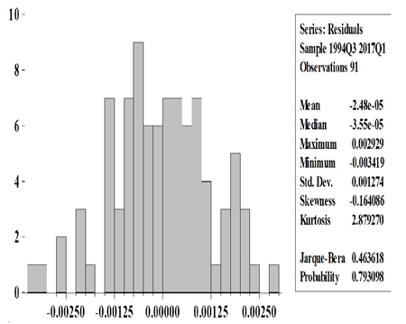
Note that, during the nowcast of the previous section, the BE models were updated according to the data revisions as well as the seasonal adjustments. This means that models are changing as needed. As an example, in table 1 I show the model estimation for the BE models with data available until July 2017, which is the latest available model from estimations made in real time (The autocorrelation analysis and the normality test are shown in appendix A3.1). Table 1 also shows how some variables could lose their significant levels (see ER t−3 , Industrial Activityt−2, ANTAD t , and EMEC t in table 1) due to data revisions and due to changes in the seasonally adjustment models, but I included those variables nevertheless, in order to keep track of them and to have comparable forecast among quarters, despite data revisions.
Table 1 Bridge equation estimation models
Variables |
BE1 |
BE2 |
||
| Coefficient |
Std. Error |
Coefficient |
Std. Error |
|
IGAEt |
.713 |
(.029) |
.746 |
(.048) |
Consumptiont−2 |
-.080 |
(.018) |
||
Industrial Activityt−2 |
.161 |
(.021) |
.059 |
(.036) |
Manufacturingt−1 |
.076 |
(.023) |
||
Importst |
.055 |
(.008) |
||
IndustryUSt |
.083 |
(.030) |
||
Constructiont−2 |
-.041 |
(.009) |
||
ANTADt |
.083 |
(.012) |
.049 |
(.029) |
ExportNoPetrolManut |
-.059 |
(.008) |
.048 |
(.010) |
ForwardIndicatort−1 |
-.270 |
(.047) |
||
BMVt |
.249 |
(.049) |
||
Cementt-3 |
-.035 |
(.006) |
.020 |
(.010) |
AMIAt-1 |
-.012 |
(.003) |
-.008 |
(.003) |
M4t-3 |
.030 |
(.010) |
||
EMECt |
.023 |
(.012) |
||
AutoPartst |
.003 |
(.001) |
||
Aluminiumt-3 |
.013 |
.002 |
||
Exportt-1 |
.053 |
(.009) |
||
Hotelt |
.034 |
(.007) |
||
Electricityt-1 |
.041 |
(.020) |
||
IndustrialGast-1 |
-.004 |
(.002) |
||
Railt-4 |
-.017 |
(.005) |
||
Tirestt-2 |
-.006 |
(.002) |
||
Moviett-2 |
-.004 |
(.002) |
||
Fuelt-2 |
-.044 |
(.016) |
||
TIIEt-3 |
-.072 |
(.028) |
||
ERt-3 |
.065 |
(.042) |
||
AR(1) |
-.647 |
(.100) |
-.434 |
(.123) |
Adjusted R-squared |
.986 |
.942 |
||
S.E. of regression |
.002 |
.002 |
||
Durbin-Watson stat |
2.088 |
2.190 |
||
Akaike info. criterion |
-9.823 |
-9.267 |
||
Schwarz criterion |
-8.967 |
-8.905 |
||
Hannan-Quinn criter. |
-9.477 |
-9.124 |
||
Note: Models shown with data available until July 31st, 2017 in order to forecast GDP growth rate of 2017-II, which was published in August 22nd, 2017.
5.2 DFM estimation
To estimate the coefficients of the DFM, I use the 11 variables of the CI-3 data set, and the maximum likelihood method (ML). In turn, the parameters of the likelihood function are estimated with the Kalman filter.9 This requires initial values for the state variables, as well as a covariance matrix to begin the recursive process. For this, I use the method suggested in Hamilton (1994b).10 The estimated state space model (the state and observation equations, respectively) is shown by equations (6) and (7), where
To use the factor(s) obtained from the estimation of the DFM (figure 2) it is necessary to make it quarterly. This is done by taking the average of the three monthly observations corresponding to each quarter
That is, the nowcast of the quarterly GDP is a linear function of the factor. The estimation procedure of this linear regression of equation (5) uses the method presented in Cochrane and Orcutt (1949) to obtain robust estimators in the presence of residual autocorrelation.

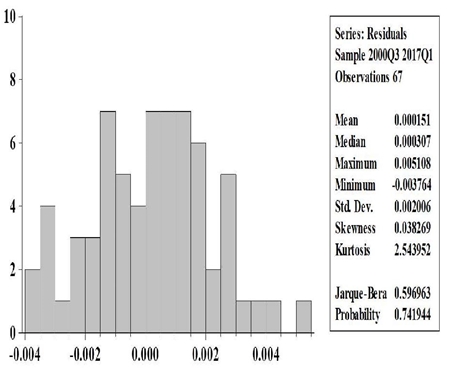
An example for the DFM estimation is shown in table 2, where data is available until July 2017. This model is the latest available from estimations made in real time (The autocorrelation analysis and the normality test are shown in appendix A3.2).
Table 2 Dynamic factor model estimation
Variables |
Coefficient |
Std. Error |
Factort |
.042 |
(.002) |
Constant |
.001 |
(.000) |
MA(1) |
-.590 |
(.113) |
Adjusted R-squared |
.871 |
|
S.E. of regression |
.003 |
|
Durbin-Watson stat |
2.040 |
|
Akaike info criterion |
-8.546 |
|
Schwarz criterion |
-8.416 |
|
Hannan-Quinn criter. |
-8.494 |
|
Note: Models shown with data available until July 31st, 2017 in order to forecast GDP growth rate of 2017-II, which was published in August 22nd, 2017.
5.3 PCA estimation
Finally, I used principle components analysis, PCA, and CI-1 and CI-2 data sets, obtaining PCA1 and PCA2 models, respectively. In the analysis I obtain all the principal components (eigenvectors), ct, that arise from each information set. However, I only consider the k components (k < n) whose eigenvalue is greater than or equal to unity, according to the criterion developed in Kaiser (1958).
After obtaining these components I rotate them in order to distribute the variance explained by each one, so I use the varimax method, which also allows me to maintain the property of orthogonality between the components even after having distributed their variance. In turn, maintaining the property of orthogonality implies a significant reduction in the number of components obtained from the high correlation between the variables considered. This helps maintain parsimony in the model that forecasts GDP growth.
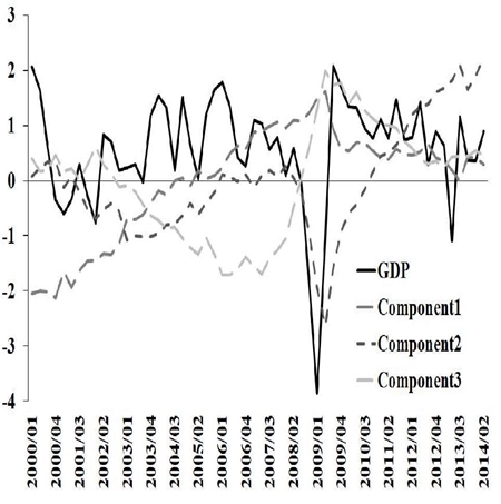
Consequently, and analogously to the methods described above, in the PCA approach, I use the k quarterly principal components (figures 2 and 3) as regressors in the following linear equation to forecast quarterly GDP growth:
where δ is an n×k matrix of coefficients,
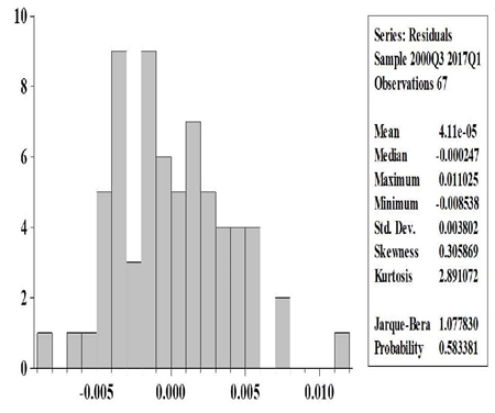
The practical example for the PCA estimation is shown in table 3, where data is available until July 2017. This model is the latest available using estimations made in real time (the autocorrelation analysis and the normality test are shown in appendix A3.3).
Table 3 Principal components analysis model estimation
Variables |
PCA1 |
PCA2 |
||
| Coefficient |
Std. Error |
Coefficient |
Std. Error |
|
Factor1t |
.079 |
(.012) |
.050 |
(.006) |
Factor1t−1 |
-.082 |
(.012) |
-.033 |
(.010) |
Factor1t−2 |
-.016 |
(.005) |
||
Factor2t |
.008 |
(.001) |
||
Factor2t−1 |
-.008 |
(.001) |
||
Factor3t |
.007 |
.003 |
||
Factor3t−1 |
-.008 |
(.003) |
||
Constant |
.005 |
(.001) |
.002 |
(.001) |
Adjusted R-squared |
.836 |
.795 |
||
S.E. of regression |
.005 |
.004 |
||
Durbin-Watson stat |
2.010 |
2.295 |
||
Akaike info criterion |
-7.597 |
-8.063 |
||
Schwarz criterion |
-7.330 |
-7.866 |
||
Hannan-Quinn criter. |
-7.489 |
-7.985 |
Note: Models shown with data available until July 31st, 2017 in order to forecast GDP growth rate of 2017-II, which was published in August 22nd, 2017.
5.4 Diebold-Mariano tests for series within sample
Under the hypothesis that the accuracy of the forecasts can be improved by taking the average or the median of the five models, I consider both of these approaches as additional forecasts. I also consider the average of BE forecasts, as well as a univariate model, AR(1), which is included as a reference. This AR model uses the quarterly GDP series as input, treating it with a logarithmic difference to induce stationarity and to approximate the GDP growth rate.
In order to evaluate the predictive power of each model and thus discern which is more appropriate to perform nowcasting, I use the modified Diebold-Mariano (DM) test proposed by Harvey, Leybourne, and Newbold (1997), hereafter referred to as the HLN-modified DM test, for small samples.11 Table 4 summarizes this test comparing each model with the rest. In the main diagonal, the mean square error (MSE) of each model is indicated in bold and the columns show which model is more accurate, according to this test. I indicate the statistical significance of error differences in each pair of compared models with asterisks. The test considers the quarters that go from 2009-I to 2016-II, the financial crisis of 2009 is included.
Table 4 HLN-modified DM test (MSE loss criterion)
Models |
AR |
PCA1 |
PCA2 |
DFM |
BE1 |
BE2 |
Mean |
Median |
Mean BE |
AR |
.808 |
||||||||
PCA1 |
PCA1 |
.665 |
|||||||
PCA2 |
PCA2 |
PCA2 |
.542 |
||||||
DFM |
DFM |
DFM |
DFM** |
.120 |
|||||
BE1 |
BE1 |
BE1* |
BE1*** |
BE1 |
.045 |
||||
BE2 |
BE2 |
BE2* |
BE2*** |
BE2 |
BE1 |
.056 |
|||
Mean (a) |
Mean |
Mean |
Mean*** |
DFM |
BE1*** |
BE2* |
.124 |
||
Median (a) |
Median |
Median |
Median*** |
Median |
BE1 |
BE2 |
Median* |
.058 |
|
Mean (BE) |
MeanBE* |
MeanBE* |
MeanBE*** |
MeanBE* |
MeanBE*** |
MeanBE*** |
MeanBE** |
MeanBE** |
.026 |
Notes: (a) = all models; p-value for statistically significance differences in MSE between compared models ***p<0.01, **p<0.05, *p<0.1 The sample includes forecasts from 2009-I to 2016-II. The mean squared error (MSE) is used as loss criterion and the uniform kernel distribution is used to compute the long-term variance.
The results of the HLN-modified DM test suggest that the forecasts generated with the DFM and with the BE models were more accurate than those obtained with the PCA2 model, but with inconclusive results with respect to the AR and the PCA1 models. Although there are no statistically significant differences between the forecast errors of the BE models and those of the DFM, there are significant differences between the forecasts of the average of BE models and the DFM.
Moreover, I find that the forecasts using this average of BE models are more accurate than those obtained with the mean or median of all the models. Indeed, those forecasts obtained the smallest MSE (MSE=0.026), which implies an error of 14 hundredths compared to the observed seasonally adjusted quarterly GDP growth (table 5). Based on these results, I conclude that the average of the BE models is the best predictor of quarterly GDP of the models analyzed.
Table 5 Forecast errors (from 2009-I to 2016-II)
Criterion |
AR |
PCA1 |
PCA2 |
DFM |
BE1 |
BE2 |
Mean |
Median |
Mean BE |
BIAS |
.001 |
.295 |
-.146 |
.035 |
-.003 |
.000 |
.036 |
.015 |
-.001 |
MAE |
.550 |
.546 |
.555 |
.243 |
.168 |
.174 |
.248 |
.165 |
.136 |
MSE |
.808 |
.665 |
.542 |
.120 |
.045 |
.056 |
.124 |
.058 |
.026 |
RMSE |
.899 |
.816 |
.736 |
.346 |
.212 |
.237 |
.353 |
.241 |
.162 |
Note: Forecast errors are calculated as the difference between the observed and the predicted value. The criteria shown in this table are detailed in section 5.5.
In order to analyze the robustness of my results, I performed the HLN-modified DM test under a different loss criterion. To do this, I use the Mean Absolute Forecast Error (MAE) as the loss criterion and a Bartlett kernel to compute the long-term variance of the differences series. The results show that the accuracy of the forecasts generated with the DFM is better than the univariate model and the PCA models, with statistically significant differences. This result is consistent with the findings of Giannone, Reichlin, and Small (2008), Rünstler et al. (2009) and Banbura and Modugno (2014), who have proposed the use of DFM when nowcasting. However, this new test strengthens my previous conclusion that the forecasts generated by all the models (including the DFM) are surpassed by the average of BE, with statistically significant differences (see appendix A5, table A3).
Furthermore, I also performed the modified DM tests on a smaller sample, one which excludes the period of the 2008-2009 financial crisis. Thus, I evaluate the forecasts from 2011-I until the end of the sample (see appendix A5, table A.4). The results favor the average of BE over any other model, with statistically significant differences (except when compared with the BE1 model, where my result is not conclusive). Again, the DFM offers more accurate forecasts than the AR and the PCA models, but the BE models produce more accurate forecasts than the former.
5.5 BE forecasts within sample
To evaluate the efficiency of the BE, I perform an analysis of the forecast errors using the following criteria, where k refers to the number of predicted periods.
Forecast Bias (BIAS):
Mean Squared Error (MSE):
Root Mean Squared Error (RMSE):
I calculated these three previously described equations using two approaches, one of rolling window and another of expanded window. In the first I estimate equation (4) with data from 1993-I to 2006-IV (
where
In the second approach I estimate equation (4) with
This implies that in the last window I perform an estimation from 1993-I to 2013-IV, with which I forecast four quarters (until 2014-IV).
Results of rolling window analysis show that the forecast errors generated with BE1 show an ascending behavior as k grows. That is, errors become larger when the forecast horizon is longer. However, this is not true for the BE2 model, where the smallest error was obtained by forecasting three forward periods. Similarly, the expanded window does not show an increase in the forecast error in any of the models (table 6).
Table 6 Forecast errors analysis in pseudo real time
Rolling window |
Expanding window |
|||||||
|
Error measure |
Forecast horizon |
|||||||
k=1 |
k=2 |
k=3 |
k=4 |
k=1 |
k=2 |
k=3 |
k=4 |
|
| BEI | ||||||||
BIAS |
.004 |
-.059 |
-.053 |
-.029 |
.017 |
-.042 |
-.040 |
-.022 |
MSE |
.118 |
.133 |
.149 |
.159 |
.117 |
.115 |
.138 |
.159 |
RMSE |
.344 |
.365 |
.386 |
.399 |
.342 |
.339 |
.372 |
.399 |
| BE2 | ||||||||
BIAS |
.021 |
.033 |
.013 |
.048 |
.076 |
.074 |
.026 |
.077 |
MSE |
.275 |
.229 |
.183 |
.353 |
.220 |
.185 |
.134 |
.229 |
RMSE |
.524 |
.479 |
.428 |
.594 |
.469 |
.430 |
.366 |
.478 |
Note: Table shows the average statistics obtained from an estimate with a rolling window and an expanded one. The size of the first window is 56 quarters in BE1 and 28 quarters in BE2; from 1993-I to 2006-IV and from 2000-I to 2006-IV, respectively.
The bias of BE1 model shows an underestimation of GDP growth as the forecast horizon grows (except in k = 4, where the bias is reduced). On the other hand, in the BE2 model with an expanded window, the bias remains relatively constant and even decreases in k = 3. These results are consistent with the findings of Giannone, Reichlin y Small (2008), who suggest the use of nowcasting to forecast one step ahead and advise against using it for future quarters.
5.6 Real-time forecasts (out of sample)
Because the BE average provides more accurate GDP forecasts than the rest of the models considered, I used it to perform a number of real-time tests in order to analyze the evolution and sensitivity of its forecast before the publication of new information corresponding to each series that belongs to the information set.
The period of study includes quarters from 2014-II to 2017-I, and the analysis consists of observing the evolution of the forecast, updating it based on the monthly release of variables that “complete” the information set. This allows us to evaluate variables to which the forecast is more sensitive and to identify the moment at which it improves its accuracy until a reliable estimate of GDP growth is obtained. Figure 4 shows an example of how the nowcasting update behaves as each of the indicators that make up the information set are published. The forecast begins with the IGAE release of data for the third month of the quarter prior to the reference one, that is, it begins during the current quarter.

I recorded my GDP growth forecasts during twelve quarters, and from these forecasts I obtained the forecast errors that were grouped by “moments”. I identified 12 moments of particular relevance that make up the real-time GDP forecast evolution for any quarter. These moments include indicators of interest that have important effects on nowcasting:
START. Publication of IGAE data; last month of previous quarter.
Publication of balance of trade data; first month of reference quarter.
Publication of car sales (AMIA) data; second month of reference quarter.
Publication of industrial activity (IMAI) data; first month of reference quarter.
Publication of balance of trade data; second month of reference quarter.
Publication of IGAE data; first month of reference quarter.
Publication of car sales (AMIA) data; third month of reference quarter.
Publication of industrial activity (IMAI) data; second month of reference quarter.
Publication of balance of trade data; third month of reference quarter.
Publication of IGAE data; second month of reference quarter.
Publication of car sales (AMIA) data; first month of following quarter. END. Publication of industrial activity (IMAI) data; third month of reference quarter.
With this information I constructed a boxplot to evaluate the speed and efficiency of nowcasting to improve its accuracy until I obtained a reliable estimate of GDP growth. Figure 5 shows the average of the forecast errors in period t(represented by a solid point) and the median of the errors (black horizontal line). The boxes in the diagram represent the dispersion limits of the forecast errors in the central quartiles and the “arms” show the forecast errors in the first and last quartiles (the hollow circles represent extreme values). The figure shows that incorporating the balance of trade data from the second month of reference quarter (moment 4) into the data set improves the accuracy of the forecast compared to that obtained with the accumulated information until the publication of the monthly indicator of industrial activity (IMAI) from the first month of the reference quarter.

Figure 5 Nowcasting forecast errors in percentage points on quarterly GDP growth (2014-II to 2017-I)
With the release of IGAE data for the second month of reference quarter (moment 9), the forecast not only approximates the true value of GDP growth, but also reduces the variance of the forecast error considerably. This means that the model I propose can offer an accurate forecast of Mexico’s GDP growth one month before INEGI publishes the official GDP data. Hence, once the IGAE data for the second month of reference quarter are included in the information set, the forecast is, on average, equal to the observed quarterly GDP growth, and 75 percent of time the margin of error is, in absolute terms, less than 0.1 percentage points of the aforementioned quarterly variation.
5.7 Bridge equations vs. specialists
As in the case of Caruso (2018), in this research I compare the forecasts of the “preferred” BE model against the INEGI rapid GDP estimations and the forecasts of the analysts surveyed by Bloomberg, as well as those of the SPF.12 However, the forecasts introduced in Caruso’s (2018) analysis are not comparable because the estimates in his DFM are not made in real time, while those of the specialists are and, moreover, he does not include the rapid GDP estimate published by INEGI.
To address the problem of data revisions, Delajara, Hernández y Rodríguez (2016) recover the historical series of GDP and those of the five indicators they included in their DFM to simulate the generation of forecasts in real time and, thus, improve the comparability with those offered by specialists.
In my case, I have a record from 2014-II to 2017-I of forecasts generated in real time with the five models that I propose in this research. As a result, I was able to compare the BE average records with the rapid GDP estimations, the median of the analysts surveyed by Bloomberg and the median of those registered in the SPF.13
Table 7 HLN-modified DM test
Models |
MeanBE |
Bloom |
SPF |
INEGI |
Mean BE |
.004 |
|||
Bloomberg |
MeanBE* |
.019 |
||
Survey of professional forecasters |
MeanBE*** |
Bloom |
.051 |
|
INEGI rapid estimation |
MeanBE* |
INEGI |
INEGI* |
.015 |
Notes: p-value for the significance of differences in MSE between compared models ***p<0.01, **p<0.05, *p<0.1. The sample includes forecasts from 2014-II to 2017-I. The Mean Squared Error (MSE) is used as loss criterion and the uniform kernel distribution is used to calculate the long-term variance. The MSE of each model is in the main diagonal in bold.
To carry out the comparison I used the HLN-modified DM test for small samples. The results of this test show that the BE model’s MSE is lower than that of Bloomberg’s forecasts, as well as the SPF’s and the rapid GDP estimations released by INEGI, with statistically significant differences. The BE model’s MSE, 0.004, indicates that during the analysis in real time, GDP growth forecast has differed, on average, 5 hundredths of the seasonally adjusted quarterly GDP variation observed (table 8), which means it offers a timely and relatively precise forecast of Mexican GDP growth rate.
6. Discussion and conclusions
In this paper, I propose a set of models to nowcast the seasonally adjusted quarterly growth of Mexico’s GDP, updating the forecasts when new information is released in the reference quarter. The forecast models that I consider are one DFM, two BE and two PCA models. I use the HLN-modified DM tests in order to evaluate the forecast errors of each model. First, the evaluation is done within sample, during the period 2009-I to 2016-II. As a reference, I include in the analysis the predictions of a univariate model (AR).
The results of the DM tests suggest that the average of the two BE models is a better predictor of quarterly Mexican GDP growth than the AR model, the DFM or the PCA models. Even compared to the mean and the median forecasts of all models (without considering the AR), the BE average is more accurate. These results were consistent under robustness checks in which I changed the loss criterion and the period of analysis. My findings contrast with those of Liu, Matheson, and Romeu (2012), who suggest the use of DFM to forecast GDP growth of emerging economies, with the exception of Mexico, where they opt for a Bayesian VAR model. However, the information set they use is substantially different from the one I propose in this document. As a preliminary explanation I suggest that the information set has such a wide variance among and within the economic variables that it is quite difficult to condense the whole information into one or a few factors. This was already noted by Gálvez-Soriano (2018) when forecasting agricultural sector growth in Mexico. This leads me to conclude that BE models are more appropriate than factor models when the dependent variable and/or the explanatory variables have relatively high variances.
In addition, I provide an analysis for predictions in real time. This was possible because I recorded the nowcasts for twelve consecutive quarters (from 2014-II to 2017-I) as new information was incorporated in each model. From this tracking I obtained the forecast errors from BE model average. My results show that the error variance declines as more information is released from the reference quarter. I also find that the model I propose in this research can offer an accurate GDP forecast a month before INEGI publishes the official National Account GDP and a week before it publishes its timely GDP estimate. Indeed, once the IGAE data for the second month of the reference quarter are included in the information set, the forecast is, on average, equal to the observed quarterly GDP variation, and 75 percent of the time the margin of error is, in absolute terms, less than 0.1 percentage points of the aforementioned quarterly variation.
Finally, I compared the nowcast with the rapid GDP estimate (INEGI), the median forecasts of Bloomberg’s analysts and with the median of the SPF, using the HLN-modified DM test. The results of the test show that the BE’s MSE is smaller than the MSE obtained from the median of the forecasts provided by the analysts surveyed by Bloomberg, and that it is also smaller than the MSE obtained from the median of the forecasts provided by the specialists who answer the SPF and the rapid GDP estimate released by INEGI. In all three cases the difference in MSE was statistically significant.