


Services on Demand
Journal
Article
 text in
  English (pdf)
 Article in xml format
 Article references
 Send this article by e-mail
Indicators
-
 Cited by SciELO
 -
 Access statistics
Related links
-
 Similars in
SciELO
Similars in
SciELO
Share

 Permalink
Contaduría y administración
Print version ISSN 0186-1042
Contad. Adm vol.65 n.2 Ciudad de México Apr./Jun. 2020 Epub Dec 09, 2020
https://doi.org/10.22201/fca.24488410e.2018.1973
Articles
Determinants of changes in gold returns
1 Universidad Anáhuac México, México
2 Universidad Panamericana, México
3 Universidad Nacional Autónoma de México, México
This paper explains the behavior of logarithmic gold returns between 1995 and 2017 by using several conditional mean and variance models that incorporate asymmetry and heavy tails effects. For this purpose, we conduct, first, an analysis based on standard autoregressive vectors in order to identify the main external regressors and, later, a sort of adjustments with different specifications of the AR-GARCH type to forecast the volatility of gold-price fluctuations. The main conclusion is that these fluctuations can be adequately explained by the behavior of the USDEER and SP500 series according to the specification AR(1)-GARCH (1, 1) that has a Student t distribution associated to it. This means that the long-term determinants of gold-return volatilities are related to exchange rate hedging strategies and anti-cyclical protection against stock markets variations by investors.
JEL code: C46; C51; D81
Keywords: Gold price fluctuations; VAR; GARCH; Risk measures; Volatility forecasts
En este trabajo se caracteriza el comportamiento de los rendimientos logarítmicos del oro entre 1995 y 2017 con base en varios modelos de media y varianza condicionales, que incorporan efectos de asimetría y colas pesadas. Para tal efecto, se lleva a cabo, primero, un análisis basado en vectores autorregresivos con el fin de identificar los principales regresores externos y, luego, una serie de ajustes con distintas especificaciones del tipo AR-GARCH para pronosticar la volatilidad de las fluctuaciones del oro con base en dichos regresores. La conclusión principal es que esas fluctuaciones pueden ser adecuadamente explicadas por el comportamiento de las series de USDEER y SP500 de acuerdo con la especificación AR(1)-GARCH(1,1) que tiene asociada una distribución t de Student. Esto quiere decir que los determinantes de largo plazo de las variaciones del rendimiento del oro están relacionados con las estrategias cambiarias y de protección contra el ciclo del mercado de valores por parte de los inversionistas.
Código JEL: C46; C51; D81
Palabras clave: Fluctuaciones del precio del oro; VAR; GARCH; Métricas de riesgo; Pronósticos de volatilidad
Introduction
There has been renewed interest in studying the behavior of gold prices because of the global financial crisis of 2007-2009. This is due to the inherent properties of this asset, which have since enabled investors to better manage their risks by building portfolios with less volatile positions. This document refers to hedging and inflationary properties, and those that derive from its functions as a value holder, safe haven, and portfolio diversifier (Baur et al., 2016). Each of these properties takes on particular importance based on the general circumstances surrounding an economy. In times of crisis, for example, the strong negative correlation between gold and some financial assets enables investors to use the precious metal, not only as a safe haven but also as a portfolio diversifier (Trück and Liang, 2012). Similarly, in times of continuous devaluations, gold is used as a value holder in different hedging strategies (Kristjanpoller and Minutolo, 2015).
This document considers the importance of these properties in the long term by studying the determinants of the price of gold in an era marked by abrupt highs and lows in the international price of the precious metal. In particular, its aim is to forecast the volatility in the variations of logarithmic gold returns expressed in U.S. dollars (USD), based on the behavior of some macroeconomic and financial factors that have differentiated impacts in the period between January 1995 and August 2017. For this, several statistical analyses are made on the series of gold returns, including adjustments of models of conditional mean and variance (AR-GARCH type) under different risk regimes. The observation window on which the forecast of volatilities and their backtesting is made represents a subsample or set of tests comprised of the last 100 monthly periods available in the period under study.
In statistical calibration, the extensions that best capture (filter) the dynamics of the volatility of the series common to the GARCH standard specification, without incurring in over-parameterization of the models, are used. For this purpose, a balance is made between the precision and the level of complexity of the GARCH specifications, based on a rigorous validation analysis of the models, as well as its conceptual relevance. On this last point it is worth noting, for example, that due to the fact that the series of monthly gold returns identify autoregressive patterns (AR) in the conditional mean, the methodology uses AR (VAR) vectors to identify the behavior of external factors or regressors according to their contribution to the volatility (uncertainty) in gold fluctuations. This is a new aspect of the work that is in line with the claims of the authors who study the co-movements of gold with other factors under the copula approach.
The conclusions of the document confirm some results that were already proven in the literature by stating that the determinants of the volatility of gold returns between 1995 and 2017 are of a widely recognized importance, as are the cases of the effective rate of the dollar and the stock indices (SP500). However, there are also other new elements that place the document as a pioneer, at least in the country, and that suggest that these determinants have a longer-term rather than a short-term influence; that the GARCH specifications present an unsurpassed performance in forecasting the volatility of commodities (such as gold), not only inside but also outside the sample; and that the calibration of AR-GARCH models is ideal for identifying the persistence of the determinants of variations in gold returns in data series divided into multiple horizons, with asymmetry problems and fat tails.
The document consists of two more sections. The second provides the general context of the problem by including a brief review of the state of the art, followed by an exploratory examination of the main characteristics of the information used (sample size and justification of the period considered), and a description of the behavior of the gold return series over time. The third section develops a calibration analysis of AR-GARCH models under different risk horizons in order to find the best predictor of out-of-sample forecasts for the selected group of factors. The conclusions discuss the main results of the document.
General Context
Determinants of the price (return) of gold in literature
Gold price determinants include real factors, both financial- and economy-related. Among them, the literature highlights the prices of other commodities (specifically silver and oil), interest rate, inflation, exchange rate, stock market volatility, consumer price index, lagging rates of industrial GDP and monetary aggregates (such as M2), news about growth expectations, and macroeconomic shocks (Poshakwale and Mandal, 2016; Pierdzioch et al., 2016). The variability of each of these factors, as well as their intricate interrelationships, make it challenging to identify the determinants of fluctuations in the price (returns) of gold, mainly because their dynamics are state-dependent and, therefore, it is not possible to establish definitive associations among them over time. The co-movements of gold with macroeconomic or financial factors change radically with periods of market stress, and this may increase or decrease the importance of some of its properties (Piplack and Straetmans, 2010). Poshakwale and Mandal (2016) point out that if these movements intensify (attenuate) in times of economic contraction, it is highly likely that the safe haven property of gold will be compromised (potentialized).
Before this scenario, the studies have taken two complementary paths to find the determinants in the change in the price (returns) of gold, following well-differentiated forecasting methodologies within (non-predictive forecast) or outside the sample (predictive forecast). The first is the identification of the factors causing the volatility of fluctuations in the price (or returns) of gold with the help of different models of the GARCH family or a mixed version of these with some heuristics, such as supervised learning methods, neural networks, or classifier algorithms. The second way is the characterization of the dependency structures of the gold co-movements and other factors, such as those mentioned above, through the use of copulas with changing regimes.
The main results in both cases argue that:
There is no consensus on the precedence of some factors over others in explaining the volatility of the fluctuations of the gold price (returns) (Pierdzioch et al., 2016). Some studies find that dollar variations affect gold prices more than other macroeconomic factors (Tully and Lucey, 2007), while others argue that the latter are the only important ones when using intra-daily data (Cai et al., 2001)
The effects of the factors are highly unstable when forecasts are implemented within the sample, due to the existence of distinctive elements in the price of commodities (Pierdzioch et al., 2016; Batten et al., 2010; Vivian and Wohar, 2012).
The models that present better adjustments vary in general aspects according to the types of forecasts and data considered. For low-frequency time series, TARCH or IGARCH specifications are excellent predictors of gold price behavior within the sample (see Trück and Liang, 2012); quite the opposite of what happens when the data are intra-daily or the forecasts are outside the sample, since in that case the introduction of GARCH models in the hidden layer of a neural network, for example, can offer better results (Kristjanpoller and Minutolo, 2015).
Unlike traditional time series analyses, copula models reveal that: gold co-movements are highly dependent on the regime under study and not just on a specific period (they depend on the presence or absence of inflation or on the differences between economic expansion or contraction phases, to mention a few cases); the importance of a determinant is a direct function of its contribution to the uncertainty of a group of variables; and the properties of gold are not unique in the sense that although the precious metal is a clear example of coverage for real estate in times of inflation, it may not be the case in times of rising interest rates (Poshakwale and Mandal, 2016).
Selection of the study period and sample size
An outstanding feature of the earlier studies is the absence of a clear distinction between short- and long-term determinants. There is no statistical treatment in the research above aimed at establishing the differences in the weight of the macroeconomic and financial factors listed above by period length. There is also no explicit reference to the permanent or temporary properties of gold that are associated with these factors. The selected period and the statistical analysis in Section III are aimed precisely at filling this gap in the literature by seeking to identify the long-term factors and, therefore, the permanent properties of gold, which determine the variations in its returns. With that idea in mind, all the sections of Figure 1, explained below, are considered, and not just their ascending or descending periods as is the regular practice in the literature. The aim is to detect the long-term determinants that survive the upward and downward trends of gold.
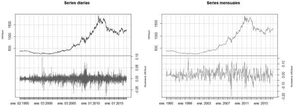
Source: own elaboration with data from Bloomberg LT (1995-2017)
Figure 1 Time series of the price (blue) and the returns (red) of the ounce of gold in USD (OROSpot) for daily (left panel) and monthly (right panel) data
The database used here is obtained from the Bloomberg LT platform (https://www.bloomberg.com/) and contains historical information on daily (5879 observations) and monthly (272 observations) closing prices for the ounce of pure gold expressed in USD (OROSpot). The observation period starts in a year of stability with low levels of international gold prices (January 1995) and ends on August 2017, once the market enters, once more, a second phase of stability, but this time with high levels in its prices. In other words, a long enough period to include all kinds of trends and levels in the middle and extremes was selected. Furthermore, periodization allows including basic series for the study of the determinants, such as the dollar effective exchange rate (USDEER) that otherwise could not be adequately contemplated. As is known, the series of this index, in particular, includes currencies of emerging economies such as the Mexican peso (MXN), the information of which is available since 1994, which is precisely the year in which the MXN adopts the free-float approach.
Characteristics of the data on gold returns
Figure 1 shows the time series of prices and logarithmic returns calculated at daily and monthly scales for the entire observation period.1 Both scales show changes in the trend and in the levels of volatility over time (intermittence).2
Concerning trends, two very distinct periods stand out: one ascending between 2002 and 2011, and the other descending from 2012 onwards (see the blue lines in Figure 1). During the first period, gold prices observed a sustained growth after the fall of stock indices, such as the NASDAQ, and the telecom crash between 2000 and 2002. The episode known as the DotCom bubble (due to its relation with information technology companies) interrupted a period of relative stability in the 1990s, when gold was seen as a value holder, to inaugurate a new bull market in which metal becomes a safe haven and an active element in portfolio diversification. At this time, there are three prominent peaks in the daily series, two small and one large, which are explained by the beginning of the Iraq war in 2003, the real estate crisis in 2008, the beginning of the European crisis in 2009 and its consequent impact on the stock market in September 2011. The second period covers the years between 2012 and 2015 and is characterized by a sustained drop in gold prices as a result of the “overheating” of the gold market that began in September 2012 (Pierdzioch et al., 2016).
In accordance with these trends, the red lines in Figure 1 present a pattern showing cumulus or alternating periods of high and low volatilities between 1999 and 2000 (with a predominantly upward peak in 1999), 2008 and 2010 (with a predominantly downward peak in 2008), and 2011 and 2013 (with symmetrical peaks upward and downward). This pattern causes very disparate OROSpot returns over time. According to Figure 2, the monthly behavior of accumulated OROSpot returns over different horizons shows strong movements in gains and losses, especially since 2005. Specifically, the maximum annualized gain occurs during 2006, while the maximum loss occurs in 2013. Other episodes of significant losses are recorded between 1997 and 1998 with the Asian and Russian crises, as well as substantial gains between 2008 and 2012 during the global financial crisis.
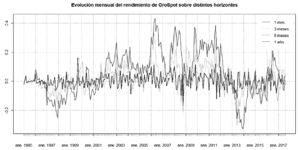
Source: own elaboration with data from Bloomberg LT (1995-2017).
Figure 2 Monthly calculation of the performance of the accumulated OROSpot over different risk horizons (mobile windows): monthly (blue), quarterly (green), semi-annual (orange), and annual (red).
Table 1 presents the main descriptive statistics of OROSpot logarithmic returns for daily, monthly, quarterly, and annual frequencies (without overlap), as well as the monthly calculation of quarterly and annual cumulative returns with mobile windows. It can be seen that the mean and median values of returns are positively larger as the observation window is expanded from days to months or years. In other words, the longer the investment horizon, the higher the mean or median gold returns. However, unlike other studies, these values are significantly lower due to the length of the period considered. For series that include only the upward trend in Figure 1, the mean daily returns are up to 2000 times larger than the one recorded in the present sample (0.04 vs. 0.0002), so these results are not always comparable with the existing literature. Compare, for example, these values with those of Trück and Liang (2012), who consider a sample between January 1999 and December 2008. Specifically, it is possible to state that the statistics of the performances of the ascending period in the price of gold are equivalent to the annualized values of Table 1, so that, the smaller the window of observation of the Table, the higher the coefficients of variation: the series of returns are more leptokurtic and the distributions of returns are less normal. The p-values reported in the last row of Table 1 for the Jarque-Bera (JB) test statistic indicate that these distributions are not normal for daily, monthly, and quarterly frequencies, at 5% significance.
Determinants of gold return fluctuations
A standard VAR model
In order to develop a methodology that characterizes OROSpot variations over different risk horizons, the following economic (real) and financial variables that have been widely highlighted in the literature are included: dollar effective exchange rate (USDEER), West Texas Intermediate oil barrel price in USD (WTI), Standard & Poor’s 500 (SP500) index, U.S. consumer price index (USCPI), U.S. LIBOR interbank interest rate (LibUSD), U.S. unemployment rate (USunEmp), and U.S. industrial production index (USIProd). The choice of each variable obeys the properties of gold, which is under research. With USDEER, the aim is to evaluate the property of gold as a decisive element of hedging. With WTI, its role as a diversifier of portfolios that include other commodities is investigated; with SP500, the quality of gold as a safe haven against the volatilities of the stock market is measured; with USCPI, its role in hedging against inflation is explored; and, finally, with the LibUSD, USunEMp, and USIProd factors the aim is to analyze its function against the volatilities of the business cycle.
Because there is no established model in the literature for forecasting gold price (returns) volatility, these variables are either used as exogenous predictors in time series models or as control variables in heuristic or copula models (Baur et al., 2016). This work follows the usual practice adopted by time-series studies of considering the factors mentioned earlier as external regressors in the explanation of variations in gold returns, regardless of their state-dependent nature (this will be addressed in the conclusions). In this sense, regressors are expected to have the sign corresponding to the activation of the property of gold, that is: a positive sign for OROSpot (seasonality), USDEER (exchange rate coverage), USCPI (inflation coverage), USunEmp (economic cycle coverage), and LIBUSD (differential rate coverage), and a negative sign for WTI (diversification of portfolios that include other commodities), USIProd (investments in the industrial cycle coverage), and SP500 (stock market cycle coverage).
The first step in determining the temporary effect that these regressors have on the OROSpot is to analyze their behavior in the reference period. Figure 3 shows that most series observe components of constant and trend effects when considering the levels of each factor. To verify the existence of unit root and to evaluate the order of integration and stationarity of the series, the Augmented Dickey-Fuller (ADF) tests, on levels and first differences, and the tests of Kwiatkowski-Phillips-Schmidt-Shin (KPSS) and Phillips-Perron (PP) are applied (see Table 2). For the OROSpot, USDEER, WTI, and SP500 variables, the logarithmic prices are taken so that the first differences correspond to the returns. The analysis considers deterministic components of constant and trend over time, as well as the effect of explanatory terms given by the lags of the variable. For a significance level of 5% it is concluded that, except for USunEmp and USIProd (whose KPSS test indicates that the assertion is valid at 1% significance), all order 1 series are integrated.
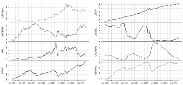
Source: own elaboration with data from Bloomberg LT (1995-2017)
Figure 3 Monthly time series of the considered global indicators.
Table 2 ADF test values for the level (with constant and trend deterministic components and two lags) and first differences (with a constant deterministic component and a backlog) series
| Variable | Deterministic components | Lags | Calculated ADF | Critical values | Calculated KPSS | Calculated PP | ||
|---|---|---|---|---|---|---|---|---|
| 1% | 5% | 10% | ||||||
|
|
|
|
|
|
|
|
|
|
Note: The critical values associated with the KPSS test statistic for the level series are: 0.22, 0.15, and 0.12 (with significance levels of 1%, 5%, and 10%, respectively); and the corresponding values for the difference series are: 0.74, 0.46, and 0.35. In the case of the PP test, the critical values associated with the calculated statistics are: -4.00, -3.43, and -3.14 (level series) and -3.46, -2.87, and -2.57 (difference series).
Source: own elaboration
The second step is to select the factors or regressors using the VAR(p) process expressed as:
where y
t
= (y
1t
, … , y
kt
)´ is the set of eventual regressors; A
i
(kxk), i = 1, … , p, are the matrices containing the coefficients subject to estimation;
u
t
is the k-dimensional error vector that satisfies the conditions that E(
u
t
) = 0, and matrix E(
u
t
Table 3 holds the coefficient estimates of the OROSpot equation according to different models of type (1) comprised of regressors and constant and trend terms, which are selected by a sequential elimination process. The models start from the most general, in which all the regressors above are incorporated, together with their constant and trend, and conclude with the most particular specification that contains the surviving factors with values. Each model has the Portmanteau and ARCH-LM tests at the foot of the Table, which confirm or reject, respectively, the null hypotheses of no autocorrelation in the residuals and of lack of ARCH effects.
Table 3 Estimates of the parameters associated with the OROSpot equation of VAR models calibrated during the sequential removal process
| Parameters | Model 1 | Model 2 | Model 3 | Model 4 | Model 5 | Model 6 | Model 7 |
|---|---|---|---|---|---|---|---|
| lag 1 OROSpot |
|
|
|
|
|
|
|
| lag 1 USDEER |
|
|
|
|
|
|
|
| lag WTI |
|
|
|
||||
| lag SP500 |
|
|
|
|
|
|
|
| lag USCPI |
|
||||||
| lag LibUSD |
|
|
|
|
|
|
|
| lag USunEmp |
|
|
|
|
|
||
| lag USIProd |
|
|
|||||
| Constant C |
|
|
|
|
|||
| Trend T (time) |
|
|
|
|
|
|
|
| Portmanteau |
|
|
|
|
|
|
|
| Univariate ARCH-LM |
|
|
|
|
|
|
|
Note: p-values are shown in parentheses, and the cases where the variable is removed due to having a value are indicated in bold.
Source: own elaboration
Table 4 presents the final results of the adjusted VAR model, in which it is shown that the coefficient estimators are robust to heteroscedasticity and serial autocorrelation (HAC), according to the Newey and West test (1987), and that the residuals do not exhibit ARCH effects. It is worth mentioning that HAC is used because the Portmanteau test in the adjusted model 7 offers unconvincing information as it did not find evidence to reject the null hypothesis of serial non-autocorrelation. Table A1 in the Annex summarizes the equations of the adjusted VAR model.
Table 4 Estimates of the parameters associated with the OROSpot equation in the adjusted VAR model (Model 7)
| Parameters | Estimate | Standard error | t-statistic | p-value |
|---|---|---|---|---|
|
|
|
|
|
|
Note: Estimates of coefficients, standard errors, t-statistics, and p-values are robust in the presence of heteroscedasticity and autocorrelation.
Source: own elaboration
In order to detect possible anomalies in the error processes associated with each VAR model equation system, Table 5 shows different multivariate tests, as well as their corresponding p-value in parentheses. The first three columns show that the residual vectors do not exhibit serial correlation (Edgerton-Shukur test), nor do they follow a normal distribution (Jarque-Bera test), although they present ARCH effects in a multivariate context on each of the considered regressors (multivariate ARCH-LM test). The latter means that, contrary to what happens with the univariate case, the first differences of the residual vectors have heteroscedasticity effects that require a special treatment through the calibration of GARCH models, as seen below.
Table 5 Validation tests on the residuals of the adjusted VAR specifications
| Multivariate test statistics | |||
|---|---|---|---|
|
|
|
|
|
Note: The p-values are between parentheses.
Source: own elaboration.
A significant aspect of Table 5 itself is the test in the fourth column, which seeks to validate the causal effects of the regressors or cause variables of model 7 (USDEER and SP500) on the OROSpot or effect variable. In this case, the following two null hypotheses are considered: a) that the set of regressors does not cause the effect variable in Granger’s sense (1969); and b) that there is a zero correlation between the effect variable and the error processes associated with the cause variables, whose p-value is between < > according to a Wald test called instantaneous causality (Lütkepohl, 2006). In both situations the null hypotheses are rejected; therefore, it is possible to state that there is causality in Granger’s sense between the variables.
With the identification of the factors and the existence of their causality, it is important to make two notes that support the robustness of the results. The first is that, in the implementation of the last test, as well as in the variance-covariance matrix of the VAR specifications, White’s (1980) HAC and HC estimators are used to ensure the statistical significance of the coefficients, respectively. Their use is unavoidable because, otherwise, there is a severe risk of making an incorrect evaluation of the determinants, as in the case of WTI, whose coefficient is significant under the estimation of standard Ordinary Least Squares (OLS) in model 7 of Table 3, but insignificant when these estimators are used. The following section will address this point.
The second note is that, when performing a decomposition analysis of the prognostic error variance for OROSpot, over 12 and 24 monthly periods, USDEER and SP500 regressors contribute at least 2% of the prognostic error variance from the initial periods (see Table 6). These figures, based on the orthogonal matrices of impulse-response coefficients, together with the fact that the variables of the adjusted model register the expected sign, constitute solid arguments to conclude that the OROSpot monthly closing price can be adequately explained by its first lag, by the first USDEER and SP500 lag, and by the trend deterministic term. The way in which these variables interact is also very useful in these forecasts since, as shown in Table 7, their correlation is mostly negative, that is, except for the SP500-OROSpot pair that presents a not significant, positive but marginal value (0.02), all other combinations are significant and close to -50%. These characteristics of the sign and the size of the correlations are critical to keep in mind because, as has already been widely documented, it favors the role of gold as an effective portfolio balancer.
Table 6 Contribution to the forecast error variance of the adjusted VAR factors
Source: own elaboration.
Table 7 Linear correlation coefficients matrix between the monthly logarithmic returns of the selected variables
| OROSpot | USDEER | SP500 | |
|---|---|---|---|
| OROSpot | 1 |
|
|
| USDEER |
|
1 |
|
| SP500 |
|
|
1 |
Note: Between parentheses are the p-values associated with a t-test that contrasts the null hypothesis of zero linear correlation with the alternative two-tailed hypothesis.
Source: own elaboration.
GARCH filtrations
Once the determinants of the marginal behavior of the OROSpot logarithmic returns have been identified, it is important to filter the series with a GARCH specification to help predict the mean and conditional variance over different periods. To this end, it is considered that p 1t = ln(OROSpot t ), p 2t = ln(USDEER t ), and p 3t = ln(SP500 t ) are the prices of the series used in the adjusted VAR model, and the validation tests in Table 5 allow establishing the causal relationships indicated in the system (2):
where the error termsu 1t , u 2t , and u 3t , with a zero mean have no autocorrelation, heteroscedasticity, and no normality in their underlying distribution. This system can be rewritten as (3) when taking the first differences of the series of logarithmic returns r it = p it - p i , t-1 , i = 1,2,3:
where
For parameters
This result makes it clear that the system equations (2) identify USDEER and SP500 returns as explanatory variables of the mean OROSpot return behavior. However, they also make it evident that endogeneity induced by the equations of the adjusted VAR model reformulated on the differences r 2t and r 3t can be translated into a possible dependence (in conditional mean) between these and v 1t , as well as into a higher serial correlation and heteroscedasticity. To deal with these problems, model (4) adopts a functional form for the conditional mean of the gold return that facilitates the correct filtering of the error term, just as the last two equations in (3) use the filtering of the USDEER and SP500 returns as external regressors in the dynamics of gold returns.
To rule out unwanted dependencies or, in other words, that variations in gold returns do not anticipate the USDEER and SP500 return series, Table A2 in the Annex shows the cross-correlation matrices, in which each entry (i,j) corresponds to the sample correlation between r i,t and r j,t-l , for the different numbers of l lags. It is observed that, when considering the critical value ±0.122 (for a two-tailed test at 5% significance under the asymptotic distribution of the linear correlation in the presence of white noise), OROSpot presents only two significant marginal correlations in lags 7 and 8. This result, together with the correlation levels observed in Tables A1, allows confirming the conclusion established in the VAR model that the USDEER and SP500 series and the first OROSpot lag anticipate gold returns and not vice versa. Furthermore, Table A2 includes the calculation of a multivariate Portmanteau statistic proposed by Li and McLeod (1981) to contrast the null hypothesis that establishes that all cross-correlations up to a certain number of lags are zero. For a significance level of 5%, the test concludes that there is no evidence to reject the null hypothesis, except in a pair of cases for lags 3 and 8 (in fact, the conclusion is valid in all lags analyzed for significance levels of 1% or less).
In order to capture the behavior of the conditional variance of
In the univariate context, it is said that the (y t ) process follows a model of conditional mean and variance if it can be expressed as:
where (z
t
) is a white noise process,
For illustrative purposes, a standard GARCH(1,1) model that incorporates USDEER, SP500, and WTI as regressors in the equations of mean and conditional variance will be used first. The purpose of this exercise is two-fold, because, in addition to starting with a base specification that allows refining the most predictive equations for the mean and variance of the regressors, it helps to prove, by other means, that the introduction of previously discarded variables such as the WTI does not affect the conclusions already reached, mainly when HAC estimators are used. In this sense, if WTI is not significant with this new specification, then it can be said that the results of the previous VAR are robust and do not depend on a particular method of adjustment.
The specification includes a first-order term for capturing the self-regressive nature observed in OROSpot returns, with the understanding that the conditional distribution of errors is normal standard. The results in Table 8 indicate that the components of the conditional variance for the OROSpot series are exclusively influenced by the structural elements of the GARCH specification used and that, as expected, only USDEER and SP500 are significant as explanatory variables of the conditional mean. The sequential elimination of the non-significant components and a general analysis of the standardized residuals allow concluding that WTI is not an external regressor of the OROSpot conditional mean equation, as corroborated by the VAR analysis.
Table 8 Estimates of AR(1)-GARCH(1,1) model parameters for OROSpot on monthly logarithmic returns of gold price in USD
| Parameters | Estimate | Standard Error | t-statistic | p-value |
|---|---|---|---|---|
| Mean equation: | ||||
|
|
|
|
|
|
| Variance equation: | ||||
|
|
|
|
|
|
Note: The estimates of the equations are obtained through maximum likelihood
Source: own elaboration
The problem now is to determine which criteria are proper to choose the best GARCH specification that marginally models the monthly logarithmic return series for OROSpot. This is no small issue, especially considering the extensive range of GARCH models used in the literature. Therefore, in order to minimize arbitrariness in the choice, the specifications that satisfy the following three criteria are considered:
C1. The coefficients of the structural terms in the equation of mean and conditional variance are significant;
C2. The statistical tests for the validation of the assumptions of the standardized residual series and model specification are satisfactory;
C3. The backtesting of the model selected in the quantile forecast for returns, and for different probability levels and risk horizons are not statistically inferior to those of competing models.
To facilitate the reading of the following tables and relate their results to equation (4) it is enough to use the notation y t = r 1t , x 1t = r 2t , and x 2t = r 3t , and consider the inclusion of the additional parameters attributed to the various GARCH specifications.
However, since only criteria C1 and C2 are considered in this section, Table 9 presents the estimates for the marginal filtrations of each series of monthly logarithmic returns of OROSpot, USDEER, and SP500.
Table 9 Estimate results of the parameters associated with the various calibrated GARCH specifications for the monthly logarithmic returns y t of OROSpot
| y t = μ+ ψ 1 y t-1 + λσ t + ρ 1 x 1t + ρ 2 x 2t + ε t | GJRGARCH (1,1): |
|||||||||||
| ε t + σ t +z t | ||||||||||||
| z t ∼ t ν,ξ (0,1) i.i.d. | GARCH (1,1): |
EGARCH (1,1): |
||||||||||
| OROSpot | Especificación | µ | ψ1 | λ | ρ1 | ρ2 | ω | α | β | γ | ξ | ν |
| AR(1)-GARCH(1,1) |
|
|
|
|
|
|
|
1 |
|
|||
| AR(1)-EGARCH(1,1) |
|
|
|
|
|
|
|
|
1 |
|
||
| AR(1)-GJRGARCH(1,1) |
|
|
|
|
|
|
|
|
1 |
|
||
| AR(1)-IGARCH(1,1) |
|
|
|
|
|
0.97 | 1 |
|
||||
| AR(1)-GARCH(1,1) in-mean |
|
|
|
|
|
|
|
1 |
|
|||
| USDEER | (x 1t ):AR(1)-GARCH(1,1) |
|
|
|
|
|
|
|||||
| SP500 | (x 1t ):GARCH(1,1) |
|
|
|
|
|
∞ | |||||
Note: The conditional mean of incorporates the monthly logarithmic returns of USDEER (x 1t ) and SP500 (x 2t ). Estimates are obtained using the maximum likelihood method. The values in parentheses are the robust standard errors based on White’s method (1982). The heading includes abbreviated general expressions on the dynamics associated with return processes and their conditional volatility σ t under each model. The results of the estimation of the individual filtering of the series of external regressors are also included (x 1t and x 2t ). In all cases, the conditional distribution used is Student’s t-distribution with ν shape and ξ parameters (the ν = ∞ value corresponds to the biased normal standard distribution). The distribution is symmetrical when ξ = 1.
Source: own elaboration
It is generally observed that the conditional variance component for the OROSpot return series exhibits less persistence than that of the USDEER and SP500 external regressors; the white noise process (z t ) associated with the OROSpot is symmetrical and shows a certain degree of heaviness in both tails, as can be observed from the shape (ν) and bias (ξ) parameters of the conditional distribution; the USDEER factor exhibits some degree of positive asymmetry with the trend to take extreme values; and, finally, the noise process associated with SP500 is normal standard (ν = ∞ ), with a negative bias (ξ < 1). Concerning the structure of the conditional mean of the logarithmic return series, Table 9 shows an autoregressive effect of order 1 for OROSpot (whose partial effect is -0.15), as well as critical negative contributions coming from the contemporary terms of the external regressors USDEER (-1.63) and SP500 (-0.23). When incorporating the contemporary effect of conditional volatility in the mean of the process of returns, a change of sign is observed in the associated partial effect (0.16), contrary to the autoregressive effect, which allows filtering the impact of periods of high volatility as increases in the expected return of OROSpot. External regressors exhibit self-regressive behavior with a positive sign (+0.11), in the case of USDEER, and a positive constant mean (+0.0083), in the case of SP500.
Regarding the calibration of structures for conditional variance, it should be noted that, under the standard GARCH specification, the autoregressive effect induced by the order 1 lag of the structural component of the conditional variance for OROSpot (0.52) is less than those recorded by USDEER (0.76) and SP500 (0.75). This effect is superior to the differentiated contribution of the first square lag of the error process on the dynamics of the conditional variance of the three series (0.19 in OROSpot, 0.12 for USDEER, and 0.22 for SP500). It should also be noted that while the coefficient that captures the leverage effect is positive for the EGARCH specification, it is not positive for GJRGARCH because the coefficient there is significantly close to zero. Finally, all adjusted models, except for the IGARCH, are stationary, even though the average persistence observed for OROSpot (0.71) is well below the most explosive patterns identified with the external regressors of USDEER (0.87) and SP500 (0.97).
Several statistical tests are presented in Table 10 to validate the assumptions of the residual series, the structural elements, and the specifications associated to each adjusted model. It can be observed that, in addition to the persistent volatility identified for each model, it can also be added that the calibrated OROSpot specifications do not present major stability problems in the parameters, due to the fact that the critical values (at significance) associated with test statistics (Nyb) are in the order of 1.89 (GARCH and GARCH-in-mean), 2.10 (EGARCH, GJRGARCH), and 1.49 (EWMA). This situation is different for USDEER and SP500 external regressors, as their corresponding critical values are 1.49 and 1.28, respectively. The levels of bias and kurtosis presented by the standardized residuals under each specification correspond to the estimates reported for the asymmetry (ξ) and shape (ν) parameters of the selected conditional distribution. On the other hand, the p-values of the HL test confirm the correct specification of the conditional distribution of the white noise process (z t ) in all cases, except for the EWMA specification.
Table 10 Statistical tests for the validation of assumptions of the GARCH specifications
| y t = μ+ ψ 1 y t-1 + λσ t + ρ 1 x 1t + ρ 2 x 2t + ε t | GJRGARCH(1,1): |
||||||||||||||||
| ε t + σ t +z t | |||||||||||||||||
| z t ∼ t ν,ξ (0,1) i.i.d. | GARCH(1,1): |
EGARCH(1,1): |
|||||||||||||||
| OROSpot |
|
|
|
|
|
|
|
|
|
|
|
|
|
|
|
|
|
| USDEER | (x 1t ) : AR(1)-GARCH(1,1) | 0.87 | 1.03 | 0.47 | 3.85 | 0.91 | 0.57 | 0.52 | 0.43 | 0.93 | 0.41 | 0.96 | 0.78 | 0.65 | 0.27 | -5.56 | 7.734E+02 |
| SP500 | (x 2t ): GARCH(1,1) | 0.97 | 0.76 | -0.88 | 4.51 | 0.21 | 0.76 | 0.61 | 0.31 | 0.66 | 0.69 | 0.07 | 0.07 | 0.87 | 0.62 | -3.65 | 5.106E+02 |
Note: For each adjusted model, the following is reported: the persistence (Pers) of the volatility; the statistics of the tests of parameter stability (Nyb) of Nyblom (1989); the bias (sk) and kurtosis (ku) of the standardized residuals; the-p-value of the non-parametric density test (HL) of Hong and Li (2005) to evaluate the degree of adjustment of the conditional distribution; the p-values associated with the Ljung-Box statistics to detect the presence of serial autocorrelation in the standardized residuals (LjB1), as well as for their square values (LjB2) and absolute values (LjBAbs); the p-values of the Engle and Ng sign bias tests (1993) to identify the type of effect in the standardized residuals of the model on changes (shocks) in volatility in the cases of positive bias (Sb), negative bias (Nb), and the associated joint test (Jsb); the p-values of the unconditional coverage (Pc) and independence (Pi) tests proposed by Christoffersen (1998) considering a 99% confidence interval on the left tail of the returns. Finally, the values of the Bayesian information criterion (BIC) and the non-standardized plausibility (Lik) are included.
Source: own elaboration
The calculation of p-values associated with Ljung-Box statistics, and which are used to validate the hypothesis of no serial autocorrelation of standardized residuals, whether nominal (LjB1), squares (LjB2), or in absolute value (LjBAbs), indicates that the filtering of returns is adequate. Similarly, most sign bias tests support the idea that there is no evidence that specifications have bias problems in capturing volatility, as except for the OROSpot series that exhibits sign bias (Sb) there are no other asymmetry problems with abrupt changes or shocks. The results of the conditional coverage test (Pc), implemented for the calculation of Value at Risk (VaR) at 99% on the left tail of the returns (within the sample), maintain that the number of observed exceptions (losses higher than VaR) is in line with the confidence level of the risk metric in all cases.
With all these results and considering the BIC and likelihood (Lik), the standard GARCH and EGARCH models are, respectively, those that have better predictive ability to model the OROSpot series.
Forecasts of multiple future periods
To marginally evaluate the performance of the GARCH filter specifications in the OROSpot forecast, as indicated in criterion C3, a global backtesting mechanism is then implemented. In other words, the conditions represented by the models in Table 9 are reproduced to forecast the monthly performance of the variables of interest over several future periods. Specifically, the analysis focuses on evaluating the forecast of quantiles in both tails of the underlying marginal distribution, for which the probability levels of 1%, 5%, 10%, 15%, 85%, 90%, 95%, and 99% are fixed. In the case of the quantiles located on the left tail of the return distribution (levels of 1%, 5%, 10%, and 15%), the number of outputs that are less than the forecast (excess) is compared with the expected number of excesses below the probability level of the quantile. For the quantiles on the right tail (levels of 85%, 90%, 95%, and 99%), the number of realized returns that are above the quantile forecast is contrasted with the expected number of excesses below the corresponding level. Both analyses are performed for each quantile and horizon from periods forward.
The number of monthly periods (M) going forward that are contemplated are: 1M, 2M, 3M, 6M, 9M, and 12M. As a criterion for readjustment of the model, it is established that every six months, the values of the parameters are recalculated according to the historical information available up to that moment. The evaluation process considers that, for each horizon and probability level, forecasts of the VaR risk metric are generated during the last 100 available monthly periods (test set) in the sample. Each forecast must be contrasted with the observed (realized) monthly return in the forecasted period (future).
To measure the degree of correspondence between quantile forecasts and realized return values, Kupiec’s (1995) unconditional coverage test was used. Table 11 reports the p-values corresponding to the statistics of that test, which, as is known, follows a chi-square distribution with a degree of freedom under the null hypothesis that states that the proportion of observed excesses is equal to the level of confidence associated with the quantile (correct coverage). Cases in which the p-value is less than the confidence level associated with the quantile (correct coverage) at a significance of 0.05 are labeled in red. To the right of each p-value is included the number of excesses observed in the tail area of the underlying return distribution. Complementarily, at the right end of the header of each table, it shows the calculation of a distance metric that measures the average level of dispersion, presented by the number of observed excesses for the number of expected excesses. This computation is made for each GARCH specification.
Table 11 Results of the implementation of Kupiec’s (1995) test on the quantile forecast of monthly OROSpot logarithmic returns under different probability levels and risk horizons (forward periods)
| AR(1)-GARCH(1,1)-t Student | 5.0 | AR(1)-EGARCH(1,1)-t Student | 6.4 | |||||||||||||||||||||
|---|---|---|---|---|---|---|---|---|---|---|---|---|---|---|---|---|---|---|---|---|---|---|---|---|
| Nivel | 1M | 2M | 3M | 6M | 9M | 12M | 1M | 2M | 3M | 6M | 9M | 12M | ||||||||||||
|
|
|
|
|
|
|
|
|
|
|
|
|
|
|
|
|
|
|
|
|
|
|
|
|
|
| AR(1)-GJRGARCH(1,1)-t Student | 5.4 | AR(1)-IGARCH(1,1)-t Student | 3.1 | |||||||||||||||||||||
| Nivel | 1M | 2M | 3M | 6M | 9M | 12M | 1M | 2M | 3M | 6M | 9M | 12M | ||||||||||||
|
|
|
|
|
|
|
|
|
|
|
|
|
|
|
|
|
|
|
|
|
|
|
|
|
|
| AR(1)-GARCH(1,1)-in-mean-t Student | 5.6 | |||||||||||||||||||||||
| Nivel | 1M | 2M | 3M | 6M | 9M | 12M | ||||||||||||||||||
|
|
|
|
|
|
|
|
|
|
|
|
|
|
||||||||||||
Note: For each horizon, the p-value of the test statistic (first column) and the number of quantile excesses (second column) observed in both tails are reported. In the upper right corner of each table, the average value is reported over the risk horizons of the Euclidean distance metric that measures the average size of the observed dispersion between the excesses made and the number of expected excesses of the quantiles (the two smallest values have been labeled in blue). Finally, the cases in which the p-value of the Kupiec statistic is less than the 5% significance level are marked in red.
Source: own elaboration
The general conclusion of the table is that, if it is considered that the number of cases in which the null hypothesis that the quantile calculation presents a correct coverage is rejected, then it is observed that the specifications with the best performance in the forecast of quantiles for the OROSpot series are AR(1)-GARCH(1,1) and AR(1)-IGARCH(1,1).
As an additional strategy to measure the performance of the GARCH specifications used to filter OROSpot returns, the calculation of the standard forecast error metrics of the conditional variance over the test set used in the backtesting exercise is performed. For this, the following sample versions of loss functions (criteria) developed by Hansen and Lunde (2005) are used:
where (h
t
) is the forecast of the underlying conditional volatility process (σ
t
). As a proxy of variance
The calculation of the MSE 1 y and MSE 2 criteria allows evaluating the error of the volatility forecast for each of the monthly horizons (1M, 2M, 3M, 6M, 9M, and 12M) under each GARCH type model used in the backtesting exercise. The test of superior predictive ability (SPA) proposed by Hansen (2005) is used to verify whether the forecasts are statistically different. In it, the null hypothesis establishes that no model is inferior to other competing models given a loss function. Table 12 shows the values obtained for the following criteria MSE 1 and MSE 2 in each GARCH specification under each forecast horizon considered. Parentheses include the p-values resulting from the application of the SPA test. The cases in which the p-value is lower than the level of significance have been marked in red. In general, there are no significant differences in the predictive capability of volatility, except for the AR(1)-GARCH(1,1) and IGARCH(1,1) specifications with horizons of 3 and 6 months, respectively. If the average values of each metric used are compared, under the criterion MSE 1 the EGARCH models have the lowest error levels. In the same sense but based on the MSE 2 criterion, the IGARCH specification keeps the error averages small.
Table 12 Forecast error metrics and under each GARCH specification on different risk horizons
| MSE 1 (x10-4) | ||||||
|---|---|---|---|---|---|---|
| 1M | 2M | 3M | 6M | 9M | 12M | |
| AR(1)-GARCH(1,1) |
|
|
|
|
|
|
| AR(1)-EGARCH(1,1) |
|
|
|
|
|
|
| AR(1)-GJRGARCH(1,1) |
|
|
|
|
|
|
| AR(1)-IGARCH(1,1) |
|
|
|
|
|
|
| AR(1)-GARCH(1,1)-in-mean |
|
|
|
|
|
|
| MSE 2 (x10-5) | ||||||
| 1M | 2M | 3M | 6M | 9M | 12M | |
| AR(1)-GARCH(1,1) |
|
|
|
|
|
|
| AR(1)-EGARCH(1,1) |
|
|
|
|
|
|
| AR(1)-GJRGARCH(1,1) |
|
|
|
|
|
|
| AR(1)-IGARCH(1,1) |
|
|
|
|
|
|
| AR(1)-GARCH(1,1)-in-mean |
|
|
|
|
|
|
Note: The values between parentheses indicate the p-value of Hansen’s superior predictive ability (SPA) (2005).
Source: own elaboration
After analyzing the validation results (Tables 9 to 12) on the aspects considered in criteria C1, C2, and C3 described above, it is concluded that the most suitable specification for filtering the monthly logarithmic OROSpot returns is the AR(1)-GARCH(1,1) model with Student’s t-distribution and external regressors USDEER and SP500.
Conclusions
This document offers enough evidence to affirm that the fluctuations in the price of gold experienced between January 1995 and August 2017 can be explained by their first lag and that of the USDEER and SP500 external regressors. The VAR analysis and the various tests used throughout Tables 9 to 12 guarantee a well-founded causality between the two factors and the OROSpot returns (and in a single direction), which makes it possible to state that gold investments are, during that period, an efficient means of hedging against exchange rate (USDEER) and stock market (SP500) volatilities.
The negligible weight of the other factors included in the sample, and whose importance is recognized in the assorted studies mentioned in the Introduction, is of a statistical nature only and should not be misinterpreted. The length of the period considered undoubtedly reduces the explanatory power of the factors discarded because it is clear that their influence is most noticeable in the ascending or descending part of the trends in Figure 1, but not in the sum of the two. Changes produced by movements in interest rates, stock bubbles, or macroeconomic shocks are undoubtedly better appreciated in the short term or under measurement schemes that include changing regimes in small sample periods. Hence, the conclusion obtained in this work should be interpreted more as a long-term result, that is, as permanent properties of gold that are added to those resulting from short-term events.
The document develops validation and backtesting on the adjusted model to support this conclusion. The first focuses on characterizing the behavior of the OROSpot logarithmic returns through the correct modeling of two dynamic components: the conditional mean (trend) and the conditional volatility. This characterization is achieved employing the AR(1)-GARCH(1,1) specification with a biased conditional t-distribution, as it is the one that satisfactorily fulfills the white noise assumptions of the standardized residuals and the adjustments of the dynamics of trend and volatility. According to this specification, the logarithmic returns of USDEER and SP500 more significantly affect the fluctuations of OROSPOT returns than their own autoregressive effect, due to their more considerable influence on the conditional mean and their higher levels of volatility persistence.
With the performance tests, the document validates that the out-of -sample forecasting ability of the selected model is not inferior to that of competing models under different risk and error metrics of the volatility forecast in 100 monthly periods. The final result is that, in general terms, there are no significant differences in the predictive ability of OROSpot volatility between the AR(1)-GARCH(1,1) and the rest of the specifications with positive performance in backtesting, so that the adjusted model complies with criterion C3.
In general, it can be said that the selection, validation, and performance stages carried out here for the adjusted model constitute a robust tool for measuring the risk associated with variations in the price of gold in USD. Portfolio managers with exposure to OROSpot fluctuations over low-frequency horizons (monthly, quarterly, half-yearly, annual) can substantially benefit from the use of the methodology developed, especially since the multivariate treatment of the standardized residual series obtained for OROSpot, USDEER, and SP500 from the GARCH filter (see Table 9) provides a solid basis for the generation of future gold price scenarios.
It should be clarified that, notwithstanding its usefulness, the proposed methodology has the limitations of concentrating on short-term (monthly-annual) risk horizons and avoiding the joint treatment of gold and other variations of regressors. For these reasons, it is convenient to suggest, as a future line of research, the study of broader risk horizons, possibly multiannual, as well as the use of meta-distributions based on multivariate copulas. The inclusion of longer horizons undoubtedly demands a greater historical depth in the sample to implement more general backtesting or changes in the structural components of the means and conditional variances that allow the effects of the world economic cycle to be incorporated. With the implementation of copulas, the proposed methodology can better characterize the joint distribution of the random vector associated to the noise processes of the dynamics of the conditional mean and variance, and, in this way, study the co-movements of gold and the other regressors in varied circumstances. Furthermore, due to the characteristics of OROS-pot performance distributions and their determinants (with heavy and asymmetric tails), the study of copulas may be a suitable vehicle for a detailed treatment of tail dependence in the underlying noise processes.
REFERENCES
Batten, J., Ciner, C., y Lucey, B. (2010). The macroeconomic determinants of volatility in precious metal markets. Resources Policy, 35, 65-71. https://doi.org/10.1016/j.resourpol.2009.12.002 [ Links ]
Baur, D., Beckmann, J., y Czudaj, R. (2016). A melting pot. Gold Price forecasts under model and parameter uncertainty. International Review of Financial Analysis, 48, 282-291. https://doi.org/10.1016/j.irfa.2016.10.010 [ Links ]
Cai, J., Cheung, Y., y Wong, M.(2001). What moves the gold market? Journal of Futures Markets 21,257-278. https://doi.org/10.1002/1096-9934(200103)21:3<257::AID-FUT4>3.0.CO;2-W [ Links ]
Christoffersen, P.F. (1998). Evaluating Interval Forecasts. International Economic Review, 39, 841-862. http://dx.doi.org/10.2307/2527341 [ Links ]
Engle, R. y V. Ng. (1993). Measuring and Testing the Impact of News on Volatility. Journal of Finance, 43, 1749-1778. http://dx.doi.org/10.2307/2329066 [ Links ]
Granger, C. W. J. (1969). Investigating causal relations by econometric models and cross-spectral methods. Econometrica, 37, 424-438. http://dx.doi.org/10.2307/1912791 [ Links ]
Hamilton, J.D. (1994). Time Series Analysis. Princeton University Press, Princeton. [ Links ]
Hansen, P.R. (2005). A test for superior predictive ability. Journal of Business & Economic Statistics, 23, 365-380. http://dx.doi.org/10.1198/073500105000000063 [ Links ]
Hansen, P. R. y Lunde, A. (2005). A forecast comparison of volatility models: Does anything beat a GARCH(1,1)?. Journal of Applied Econometrics, 20, 873-889. http://dx.doi.org/10.1002/jae.800 [ Links ]
Hong, Y. y Li, H. (2005). Nonparametric specification testing for continuous-time models with applications to term structure of interest rates. Review of Financial Studies, 18(1), 37-84. https://dx.doi.org/10.1093/rfs/hhh006 [ Links ]
Johansen, S. (1995). Likelihood Based Inference in Cointegrated Vector Autoregressive Models. Oxford University Press, Oxford. [ Links ]
Kristajanpoller, W. y Minutolo, M. (2015). Gold price volatility: A forecasting approach using the artificial neural network-GARCH model. Expert systems with applications, 42, 7245-7251. http://dx.doi.org/10.1016/j.eswa.2015.04.058 [ Links ]
Kupiec, P. (1995). Techniques for Verifying the Accuracy of Risk Management Models. Journal of Derivatives, 3(2), 73-84. http://dx.doi.org/10.3905/jod.1995.407942 [ Links ]
Lütkepohl, H. (2006). New Introduction to Multiple Time Series Analysis, Springer, New York. http://dx.doi. org/10.1007/978-3-540-27752-1 [ Links ]
Newey, W. y West, K. (1987). A simple positive semidefinite, heteroscedasticity and autocorrelation consistent covariance matrix. Econometrica, 55, 863-898. http://dx.doi.org/10.2307/1913610 [ Links ]
Nyblom, J. (1989). Testing for the constancy of parameters over time. Journal of the American Statistical Association, 84, 223-230. http://dx.doi.org/10.1080/01621459.1989.10478759 [ Links ]
Pierdzioch, C., Risse, M., y Rohloff, S. (2016). A boosting approach to forecasting the volatility of gold-price fluctuations under flexible loss. Resources Policy, 47, 95-107. http://dx.doi.org/10.1016/j.resourpol.2016.01.003 [ Links ]
Piplack, J. y Straetmans, S. (2010). Comovements of different asset classes during market stress. Pacific Economic Review, 15, 385-400. https://doi.org/10.1111/j.1468-0106.2010.00509.x [ Links ]
Poshakwale, S. y Mandal, A. (2016). Determinants of asymmetric return comovements of gold and other assets. International Review of Financial Analysis, 47, 229-242. https://doi.org/10.1016/j.irfa.2016.08.001 [ Links ]
Sims, C. (1980). Macroeconomics and Reality. Econometrica 48 (1), 1-48. http://dx.doi.org/10.2307/1912017 [ Links ]
Trück, S. y Liang, K. (2012). Modelling and forecasting volatility in the gold market. International Journal of Banking and Finance, 9 (1), 48-80. https://doi.org/10.1016/j.eswa.2015.04.058 [ Links ]
Tully, E. y Lucey, B. (2007). A power GARCH examination of the gold market. Research in International Business and Finance, 21, 316-325. https://doi.org/10.1016/j.ribaf.2006.07.001 [ Links ]
Vivian, A. y Wohar, M. (2012). Commodity volatility breaks. Journal of International Financial Markets, Institutions and Money, 22, 395-422. https://doi.org/10.1016/j.intfin.2011.12.003 [ Links ]
White, H. (1980). A heteroscedasticity consistent covariance matrix estimator and a direct test for heteroscedasticity. Econometrica, 48, 827-838. http://dx.doi.org/10.2307/1912934 [ Links ]
White, H. (1982). Maximum likelihood estimation of misspecified models. Econometrica, 50 (1), 1-25. http://dx.doi.org/10.2307/1912526. [ Links ]
1Returns are calculated on a daily (d) and monthly (m) basis according to the expression:
2The monthly realized volatilities (RV) are estimated as
Annex
Table A1 Estimated parameters of the VAR model from Table 4
| t | ln(OROSpott-1) | ln(USDEERt-1) | ln(SP500t-1) | |
|---|---|---|---|---|
| ln(OROSpott) |
|
|
|
|
| ln(USDEERt) |
|
|
|
|
| ln(SP500t) |
|
Note: Standard errors are presented in parentheses. The coefficients with a value were estimated. If a 10% significance level is considered, ln(OROSpott-1) has a partial effect equal to 0.012 on ln(SP500t-1). However, this does not affect the conclusions derived from the adjustment of the VAR model.
Source: own elaboration
Table A2 OROSpot, USDEER, and SP500 cross-correlation matrices of OROSpot, USDEER, and SP500 returns
| Lag 1 | Lag 2 | Lag 3 | Lag 4 | Lag 5 | ||||||||||
|---|---|---|---|---|---|---|---|---|---|---|---|---|---|---|
|
|
|
|
|
|
|
|
|
|
|
|
|
|
|
|
| Lag 6 | Lag 7 | Lag 8 | Lag 9 | Lag 10 | ||||||||||
|
|
|
|
|
|
|
|
|
|
|
|
|
|
|
|
|
|
|
|
|
|
|
|
|
|
|
|
||||
Note: The top panel contains cross-correlation matrices for cases of one to ten lags. For each number of lags , the entry of each sub-matrix corresponds to the sample estimate of the linear correlation between the series of returns and , where the values of the indices correspond to OROSpot, USDEER, and SP500, respectively. The bottom panel presents the calculated value for the test statistic proposed by Li and McLeod (1981) to contrast the null hypothesis that the cross-correlation matrices of up to the considered lag order are identical to the zero matrix. The corresponding p-value i
Received: March 20, 2018; Accepted: September 14, 2018
 Este es un artículo publicado en acceso abierto bajo una licencia Creative Commons
