Introduction

“An estuary is a semi-enclosed body of water with a free connection to the sea, where fresh water derived from land drainage measurably dilutes water from the ocean” (^{Pritchard 1967}). Bathymetry, wind, temperature, relative humidity, solar radiation, precipitation, and the position of lagoons with respect to the direction of river discharge determine the circulation patterns, salinity intrusions, and temperature variations in an estuary. Estuarine ecosystems are important for the development of nearby settlements, recreational activities, expansion of scientific knowledge, and the survival of endemic species and other species that spend part of their life cycle in these systems. These ecosystems produce high amounts of land-sea nutrients, and vegetation and system dynamics in them act as a natural buffer between the sea and land.

For the diagnosis of estuarine circulation, we need to take into account the dynamic behavior of an estuary under the ordinary dry and rainy seasons and how this behavior relates to the most significant forcing agents (tide, river discharge, wind, temperature, salinity, and bathymetry of the estuary). Shallow estuarine lagoons present zones where velocity magnitudes are very low, and water circulation in the system will therefore be influenced mainly by pressure gradients, bottom shear stress (friction), surface wind stress, and, for lagoons that are wider than the Rossby radius of deformation, the Coriolis effect (^{Gill and Rasmusson 1983}). An analysis of the momentum equation, which requires an analysis of barotropic pressure caused by variations in sea level and an analysis of baroclinic pressure, is performed to study water movements in the system. Some results have demonstrated that substantial gravitational circulation can develop in shallow, weakly stratified estuarine lagoons (^{Jian and Li 2012}).

The diagnosis of estuarine circulation consists in analyzing field measurements including salinity, tidal phases, flux velocity, transport (flux per unit area), and bathymetries (^{Carlin et al. 2016}, ^{Xu et al. 2017}). To completely characterize an estuary, numerical models allow obtaining current circulation patterns must be applied (^{Panda et al. 2013}, ^{Gonzalez-Vazquez et al. 2018}). Both studies are complementary in the diagnosis of estuarine circulation because, even though circulation can be inferred from well-designed field experiments, at present it is not possible to monitor all temporal variabilities of currents all around the system. On the other hand, while numerical models allows us to obtain the temporal and spatial variabilities of currents throughout the system domain, the information provided by field surveys is important for the calibration and validation of the circulation patterns obtained with numeric models.

Many numerical circulation models can be applied for estuaries (^{Salas-Monreal et al. 2018}), with some sing tracers or pressure gradients in the system (^{Mahanty et al. 2016}). More recently, three-dimensional (3D) models have been used to determine hydrodynamic behavior with free-surface, velocity, and salinity conditions associated with the dry and rainy seasons in the site (^{Zhu et al. 2015}, ^{Barrios-Piña et al. 2016}).

Mean circulation and stratification are fundamental factors in the transport of nutrients, contaminants, and fish larvae in estuarine systems (^{Paerl et al. 1998}, ^{Werner et al. 1999}, ^{Vargas et al. 2017}). The Venice System Scheme (The Venice System… 1958) is used to regionalize an estuary according to salinity levels; this scheme sections the estuary into 5 region types that provide an ecological characterization of the system according to the following salinity scales: limnetic (freshwater region, <0.5), oligohaline (0.5 to 5.0), mesohaline (5 to 18), polyhaline (middle region, 18 to 25; lower region, 25 to 30), and euhaline (30 to 35).

Estuaries can be considered shallow bodies of water that are associated with tidal phases, wave forces, and flux velocities; therefore, equations for shallow waters can be adequate to study estuaries. However, a variating condition of vertical density as a product of saline waters from the sea and fresh water from river discharges is necessary for circulation analyses. This condition is essential for the hydrodynamic circulation and salinity in the system. Therefore, the study must consider the vertical variation of salinity to establish saline intrusion conditions along the profiles of the river and the lagoon system, and changes in density and temperature (^{Lesser et al. 2004}).

This study analyzes a 3D hydrodynamic model (Delft3D, ^{Roelvink and van Banning 1995}) to estimate water circulation conditions in the Boca del Río Estuary (Veracruz, Mexico), taking into account that, even in the shallow waters of the Mandinga Chica Lagoon and Mandinga Grande Lagoon, the circulation will be influenced by baroclinic and barotropic pressure gradients. Though in the field data the system shows a uniform salinity condition throughout most of the system and a dominance of shallow conditions, the implementation of a 3D model is fundamental due to interactions with the open sea at the mouth of the system and density variations, which influence barotropic and baroclinic pressure in the estuary.

Materials and methods

Study area

The system is formed by the Jamapa River, the estuary, the Mandinga Chica Lagoon, and the Mandinga Grande Lagoon. The system is located between 18º58ʹN and 19º06ʹN and 96º01′W and 96º08′W, in Boca del Río, Veracruz, Mexico (Fig. 1).

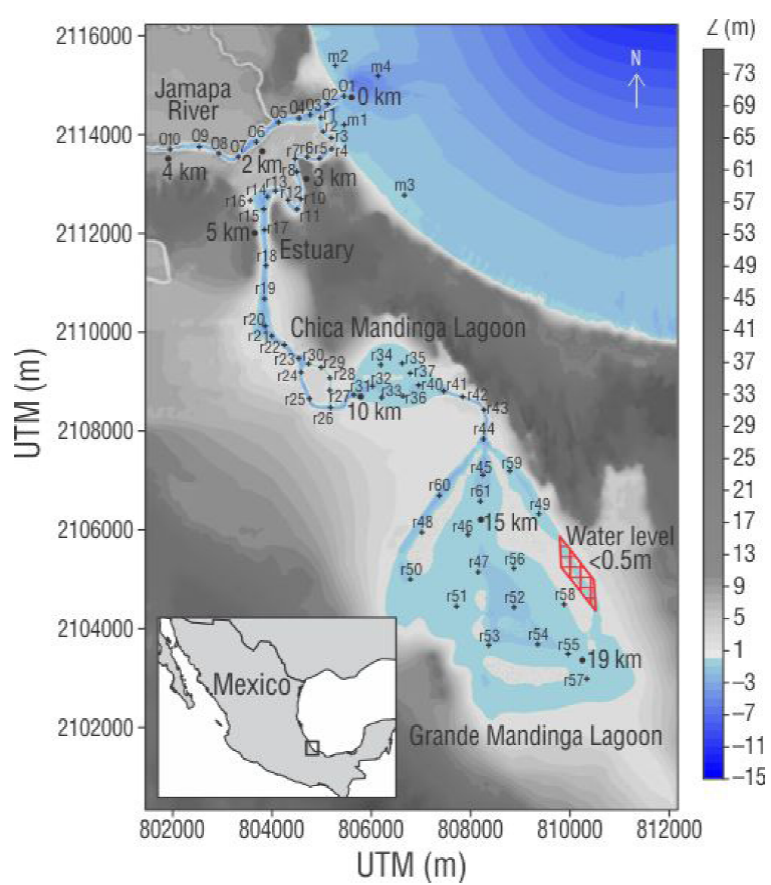
Figure 1 Study area and control stations (+). Circles indicate the length of the system from the breakwaters. The red square indicates water level under 0.5 m. 

The estuary extends over an area of 2.13 km² with an island formed at the mouth of the Mandinga Chica Lagoon; the island has an area of 0.27 km². The estuary is a 9.18-km long meandering channel with an average depth of 3 m. The Mandinga Chica Lagoon has an area of 1.72 km² and a perimeter of 5.13 km; the lagoon entrance has a maximum depth of 22 m, whereas the inner lagoon has a maximum depth of 0.9 m. A 2-km long channel with depths of 2.08-3.27 m connects Mandinga Chica Lagoon with Mandinga Grande Lagoon. The Mandinga Grande Lagoon has an area of 16.24 km², a perimeter of 17.13 km, and an average depth of 0.8 m. The water flux in the lagoon system depends solely on the discharge of the Jamapa River and the connection with the open sea; there is no relevant surface runoff in the area. The Jamapa River is the main channel of the system. During the dry season, average flux is 14.2 m³·s^-1; during the rainy season, average flux is 135.7 m³·s^-1. The average flux reached values higher than 1,000 m³·s^-1 due to extreme weather conditions during Hurricane Karl in 2010 (^{CONAGUA 2012}, ^{Riveron-Enzastiga et al. 2016}, ^{González-Vázquez et al. 2018}).

Analysis

The study area was integrated by the bathymetry obtained in the field with an echosounder and the topography plug-in of the Mexican Elevation Continuum (CEM, for its acronym in Spanish) in UTM (Fig. 1). The river within the study area has a length of 5 km upstream from the river mouth. The analysis of the estuary in the numerical model considers the forcing agents, a regular grid, and a 3D system with 5 levels determined by depth every 20%, E1 at the free surface and E5 at the bottom. The forcing agents considered were the tide, the Jamapa River discharge, temperature, and density.

The tide is the forcing agent on the seaside. This is formed by components M₂, N₂, K₁, K₂, P₁, O₁, and S₂ with amplitude values in meters of M₂ = 0.089, N₂ = 0.023, K₁ = 0.156, K₂ = 0.006, P₁ = 0.049, O₁ = 0.153, and S₂ = 0.026 and phases in grades of M₂ = 71.17, N₂ = 59.41, K₁ = 289.36, K₂ = 55.76, P₁ = 290.99, O₁ = 289.84, and S₂ = 68.58 (SEMAR 2010, ^{Salas-Monreal et al. 2019}). K₁, O₁, and M₂ show the highest amplitudes; therefore, the tide can be considered to be diurnal with average high water of 0.478 m and average low water of 0.133 m using as reference the tidal datum of the Mean Lower Low Water (MLLW) and 0.0 m elevation.

For the Jamapa River discharge, the second forcing agent, records of hydrometric stations were analyzed (^{CONAGUA 2012}). Daily records were used to determine monthly averages and the most representative ordinary conditions. Average flux values were 14.2 m³·s^-1 in the dry season (April); whereas, average flux values were 135 m³·s^-1 in the rainy season (September). A typical year had to be determined to apply the forcing agent to the system. Average values and historical records (1951-2014) were used to determine a typical year as the year with the least standard deviation. The year 2006 was the most adequate and April and September 2006 were modeled (Fig. 2a, b).

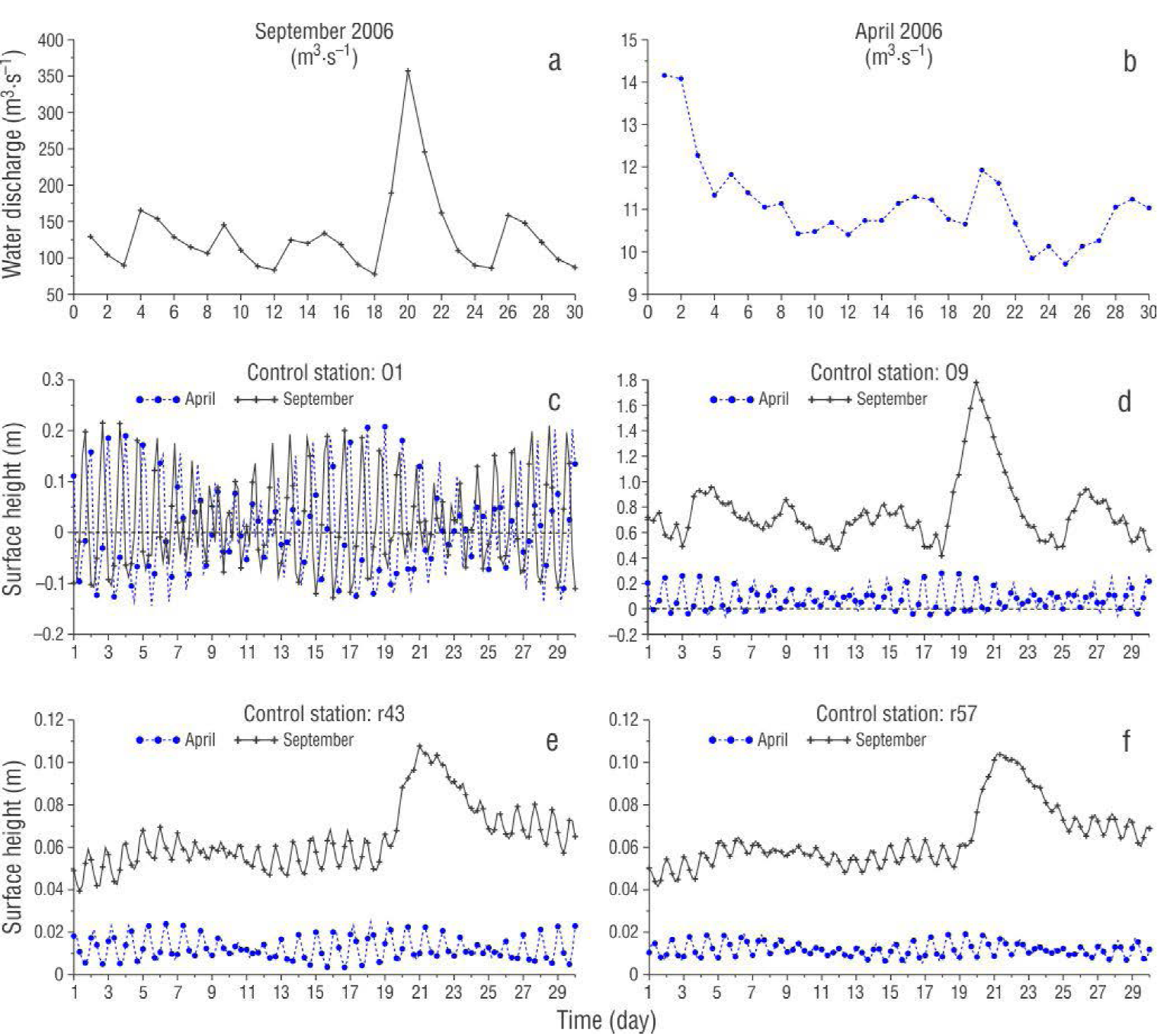
Figure 2 Daily average flux for the Jamapa River during the (a) rainy season and (b) dry season. Height of the water surface at stations (c) O1, (d) O9, (e) r43, and (f) r57, for each season. 

Variations in the temperature and the salinity gradients these induce are observed in periods of months and seasons and depend on the water temperature of the adjacent sea. This is transmitted through convection forced by the exchange of saline water volumes between the sea and lagoon, due to the tide; by seasonal fluctuations of solar radiation; and by seasonal fluctuations of convection forced by freshwater discharged by the river (^{Farreras 2006}). In April, the approximate temperature and salinity in the water of the lagoon system were 28 ºC and 30, respectively; whereas, in September the temperature and salinity were 31 ºC and 8, respectively. The records were obtained from the entrance of the Mandinga Grande Lagoon.

The DELFT3D model was applied to all historical records and some data collected in the field such as bathymetry and temperature variations in the lagoon, river, and sea. Roughness parameters were obtained from ^{Chow (1959)}. Physical parameters were obtained from the reference manual ^{Hydraulics Deltares (2006)}.

Results

The analysis of the results of the numerical model refers to April as the dry season and September as the rainy season. Variations on the free surface were analyzed according to the control stations O1, O9, r43, and r57 (Fig. 1). Station O1, located at the river mouth to the open sea, presented very similar water variations during dry and rainy seasons, with maximum and minimum values between 0.20 and -0.15 m, respectively (Fig. 2c). Station O9, located ~4 km upstream from the mouth on the Jamapa River, showed a variation of the free surface from 0.20 m to -0.05 m during the dry season, caused by the tide. During the rainy season, the variation of the free surface was dominated by river discharge not the tide and behaved similarly to the hydrogram of September with minimum and maximum values of 0.4 m and 1.8 m, respectively (Fig. 2d). Stations r43 and r57 (Fig. 2e, f), located at the entrance and end of the Mandinga Grande Lagoon, respectively, showed that the variation of the free surface behaved similarly to the tide. Flux variations caused a superelevation of 2 cm during April and 10 cm during September in the Mandinga Grande Lagoon. The lagoon behaved similarly to the River Jamapa discharge when river discharge increased during September. The system showed a 36-h delay between the flux entrance to the system and the flux entrance to the Mandinga Grande Lagoon.

Two sections along the estuary were used to analyze velocity: one in the river and one in the lagoon. In dry conditions, the Jamapa River showed velocities from 0.0 to 0.2 m·s^-1. The river showed important velocity variations in magnitude and direction from the mouth of the system to 1.5 km upstream caused by the tide (high water and low water); variations were dominated by the inflow of sea waters with a magnitude of 0.1 m·s^-1 at the bottom with an estuary-ward direction, a magnitude of 0.2 m·s^-1 with a seaward discharge direction at the surface, and a magnitude that tended to zero in the middle of the profile, which showed a typical estuarine circulation. Therefore, the tide dominated the river in the first 1.5 km during the dry season. Further upstream, the flux showed a magnitude of 0.10 m·s^-1 with a seaward discharge direction; this condition was uniform throughout depth levels and for both types of tide (Fig. 3a, c).

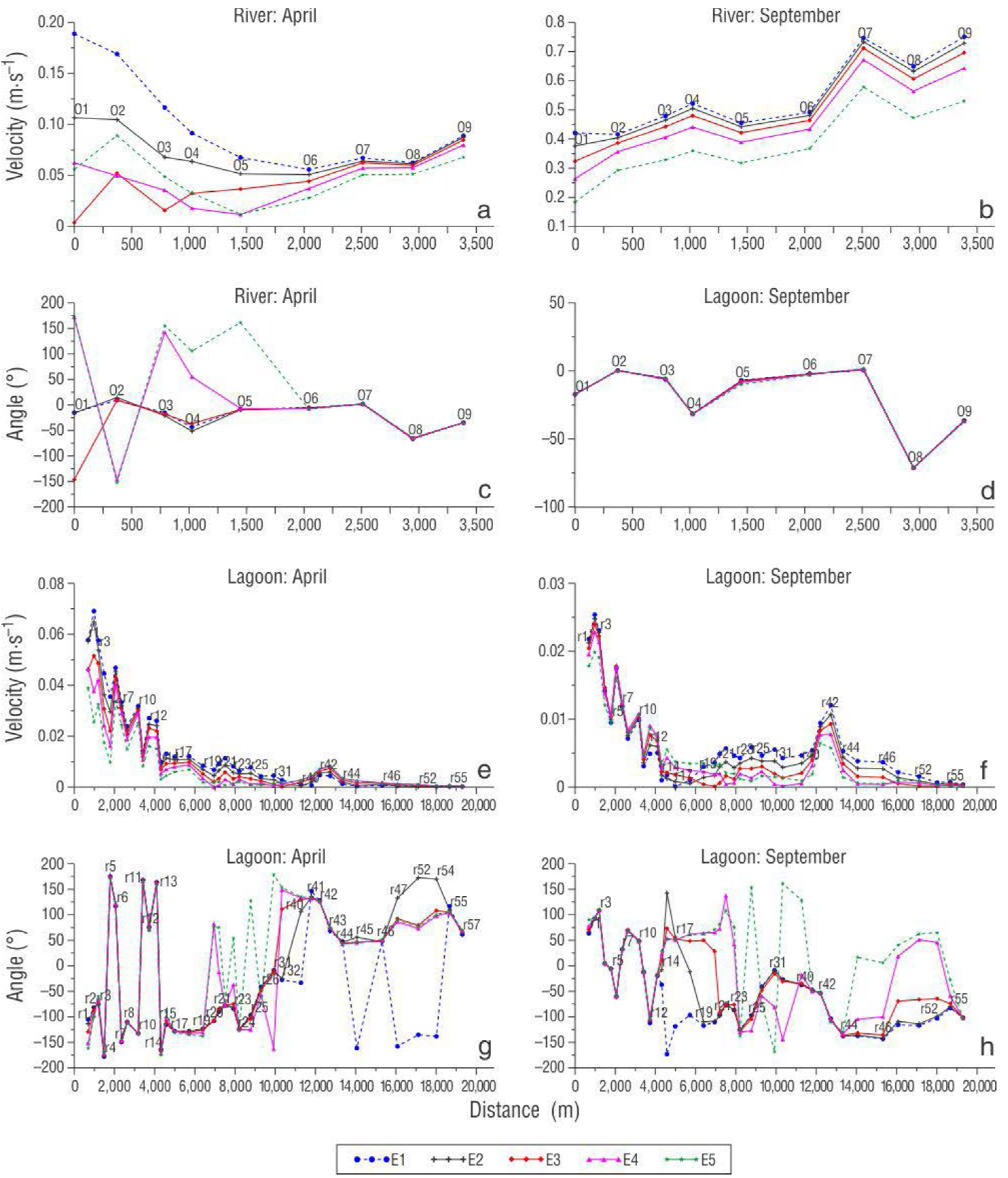
Figure 3 Model output: Velocity (a, b, e, f) and velocity direction (c, d, g, h). Water surface (E1), bottom layer (E5); positive angle indicates entrance to the system. 

In September, the river showed a more consistent behavior throughout its domain, from the mouth to 3.5 km upstream, with a velocity of 0.8 m·s^-1 and a seaward direction. For this season there was no inflow of seawater during either type of tide, which indicated that there were no saline water intrusions to the river during the rainy season (Fig. 3b, e). The second section, which was located in the lagoon system and measured ~19 km in length from the estuary entrance to the Mandinga Grande Lagoon, showed, in dry conditions, an irregular behavior up to 4 km upstream from the estuary entrance, with maximum velocities of 0.06 m·s^-1 with a uniform direction at all depth. From 4 km onward, velocities showed a regular flux throughout all depth levels, but varied in direction; the system is more regular up to the Mandinga Grande Lagoon, where depth levels showed inverted directions with near to zero velocities (Fig. 3e, g). During the rainy season, the Mandinga lagoons showed lower velocities than during the dry season, barely reaching 0.03 m·s^-1, in spite of the non-uniform fluxes observed on all depths levels in the first 4 km of the section. Velocity increased because the cross-section between the lagoons decreased; then, the velocity decreased because the cross-sectional area of each lagoon increased. From the entrance of the Mandinga Grande Lagoon, at kilometer 13, the velocity decreased to near zero (Fig. 3 f, h).

Flux increased between 18 and 24 September and caused a superelevation of 10 cm in the Mandinga Grande Lagoon; however, the variation of the velocity was minimum, whereas in the zone of breakwaters (station O1, Fig. 1) velocity values reached 0.8 m·s^-1 (Fig. 4a-d). The relation Qsea/Qriver was used to determine the dominant effect in the estuary between the river discharge and the inflow from the sea; cross-sections were used to evaluate the fluxes in the sections. The relation Qsea/Qriver showed that the river discharge dominated the system in September, whereas the tide dominated the system in April.

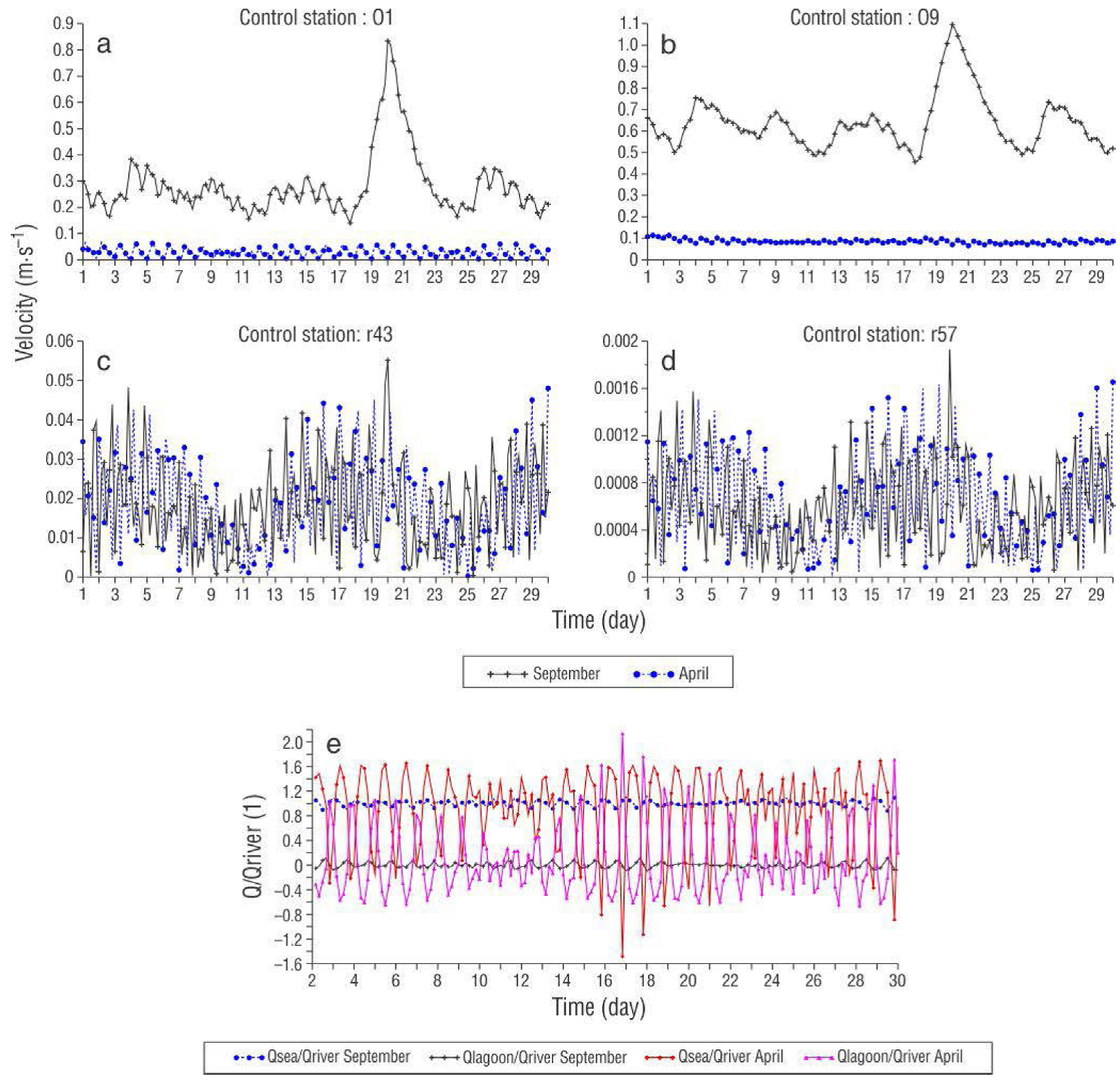
Figure 4 Average flow velocity at control stations: (a) O1, (b) O9, (c) r43, (d) r57. (e) Water-discharge relation. 

A bidimensional analysis of velocities showed that in dry conditions maximum velocities in the system were 0.10 m·s^-1 at the surface with a seaward direction and 0.05 m·s^-1 at the bottom with an inward direction; this behavior persisted for every phase of the tide. Velocity magnitudes were greater between the entrance to the lagoon and the discharge to the sea, and decreased toward the inner estuary and upstream (Fig. 5a-d). The system showed a uniform behavior at all depth levels with a constant seaward discharge during rainy conditions. Even during high water and with flux toward the inner estuary, the Jamapa River discharge inhibited the entrance of the tide and the river flux dominated circulation in the lagoon system (Fig. 5e-h).

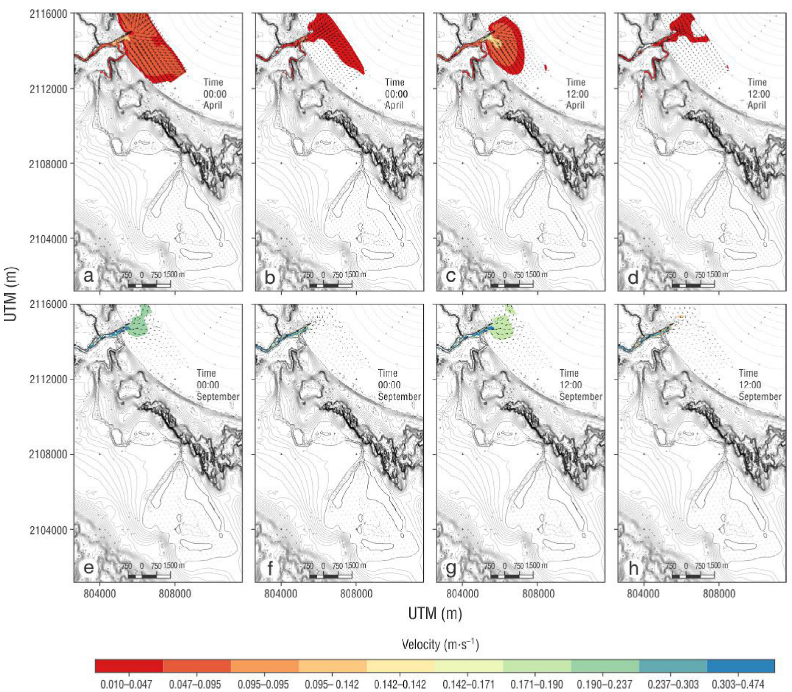
Figure 5 Velocity magnitude and direction. E1 indicates the free surface layer and E5 the bottom layer. Dry season: (a) E1 during high water, (b) E5 during high water, (c) E1 during low water, (d) E5 during low water. Rainy season: (e) E1 during high water, (f) E5 during high water, (g) E1 during low water, (h) E5 during low water. 

At station O1, the seaward river discharge showed salinity values of 23 at the surface and 33 at the bottom during dry conditions (Fig. 6a). Whereas, salinity values were 4 at the surface and 20 at the bottom during rainy conditions; mixing during this condition decreased because the Jamapa River flux increased (Fig. 6b). Salinity values tended to zero when river flux increased; this was observed between 19 and 21 September, when river discharge reached values >300 m³·s^-1 (Fig. 6b).

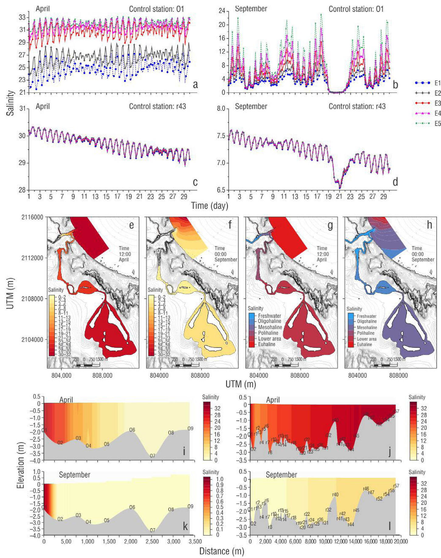
Figure 6 Salinity by layer (E1-E5) at O1 during (a) dry season and (b) rainy season and at r43 during (c) dry season and (d) rainy season. 2D salinity at E5 during (e) dry season and (f) rainy season. Classification Venice System Scheme for (g) dry season; (h) rainy season; (i) profile of salinity in the river, dry season;(j) profile of salinity in the lagoon, dry season; (k) profile of salinity in the river, rainy season; (l) profile of salinity in the lagoon, rainy season. 

Inside the Mandinga Grande Lagoon, during the dry and rainy seasons and with all phases of the tide, salinity values were uniform at all depths levels as a result of intense mixing and homogenization of the system caused by flux exchange in the narrowest sections, temperature, and flux direction changes (Fig. 6c). Salinity in the lagoon decreased because the river flux increased and caused the flux from the tide to decrease (Fig. 6d). Salinity tends to decrease in the Mandinga Grande Lagoon during dry and rainy periods because any flux from the river dilutes salinity. A bidimensional analysis of salinity in the Jamapa River showed that in dry conditions salinity tended to zero 2 km upstream, whereas in rainy conditions values were zero 0.5 km upstream from the boundary with the sea (Fig. 6e, f). Salinity increased the most during the dry season and expanded into the inner part of the Mandiga Grande Lagoon with salinity values of 30. During the dry season, the flux entered predominantly from the sea and caused higher salinity values (Fig. 6e). During the rainy season, salinity decreased to 8 in the Mandinga Grande Lagoon (Fig. 6f).

Longitudinal sections of salinity during the dry and rainy seasons showed a constant value at all depths; only at the breakwaters, where the river interacts the most with the sea, was there a significant variation (station O1). Temperature variations tend to form density and convection gradients forced by water exchange; this causes water to mix in the system and density to vary in shallow zones. Temperature variations in shallow zones together with the near-zero velocity in the lagoons caused density variations (Fig. 6i-l).

The system was classified using the Venice System Scheme (^{The Venice system… 1958}) to determine the condition variability of the circulation and stratification associated with the behavior of the lagoon during dry and rainy seasons. During the dry season, the system reached euhaline values and was apt for marine fish; during the rainy season, the system showed mesohaline values, which made it a markedly low-salinity system apt for freshwater organisms.

Discussion

Velocity conditions tend to be near zero soon after entering the lagoon system, which indicates that the system has low mobility. An analysis of the momentum equation (^{Jian and Li 2012}) is done to determine circulation:

where u, v, and w are the velocity components, η is the free surface elevation, ρ ; is density, τ _xz is the Reynolds shear stress, f is the Coriolis parameter, τ_b is shear stress at the bottom (friction), and τ_s is the shear stress at the free surface (wind stress); the terms from left to right represent the following forcings: barotropic pressure gradient, baroclinic pressure gradient, shear stress at the surface, shear stress at the bottom, Coriolis effect, and advection. For the present study, the forcing agents in the system are the river and tide fluxes; the wind and the Coriolis effect were not considered. The analysis was done at 1 m depth, which is the depth of the Mandinga Grande Lagoon; hence, the momentum equation can be re-written as follows:

Two analyses of the momentum equation (eq. 3) were done, one for the dry season and one for the rainy season for the section of the lagoon system. For the dry season, salinity values were near 30 and 0.02 m above MLLW at Mandinga Grande Lagoon. From the momentum equation, it was determined that fluxes moved due to a baroclinic condition caused by a horizontal density gradient between the breakwaters (station O1) and the Mandinga Grande Lagoon (Fig. 7a-d). During the rainy season, with salinity values of nearly 5 and elevation of the breakwater zone at 1.02 m, variation of horizontal density was limited by the discharge of the Jamapa River, which reduced baroclinic pressure; however, the increase in river flux increased horizontal variation in the free surface and thus caused a greater inclination, which produced a greater barotropic pressure condition (Fig. 8).

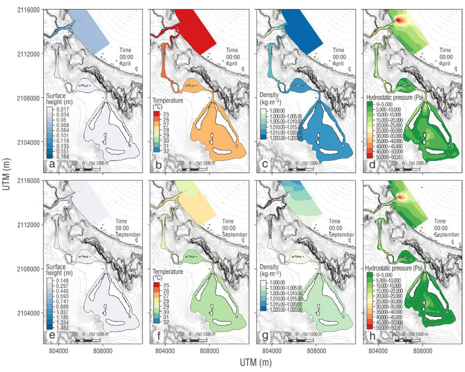
Figure 7 (a) Surface height, (b) temperature, (c) density, and (d) pressure during the dry season. (e) Surface height, (f) temperature, (g) density, and (h) pressure during the rainy season. 

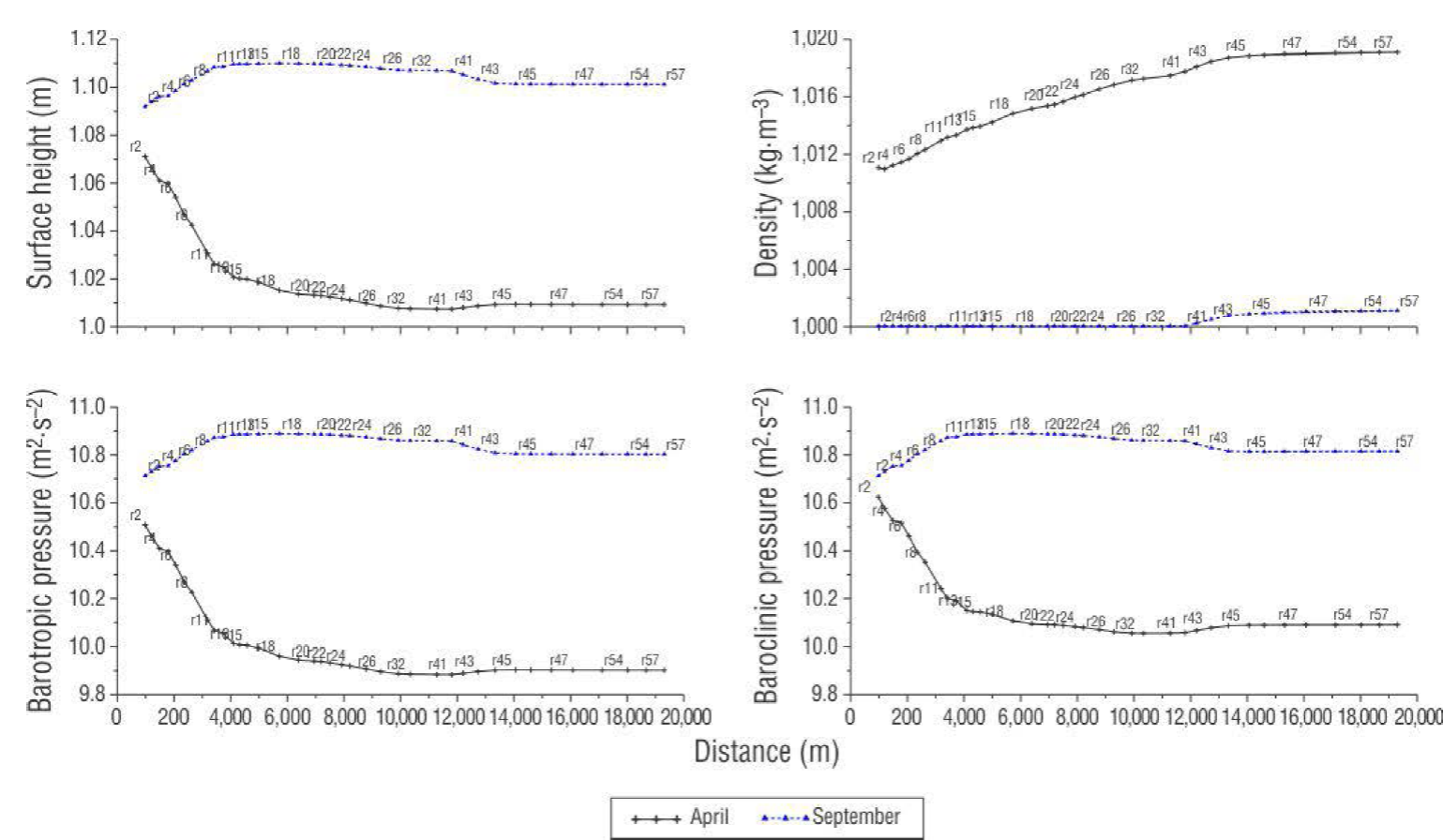
Figure 8 (a) Free surface height, (b) density, (c) barotropic pressure, and (d) baroclinic pressure. 

The circulation in the lagoon system was affected directly by variations in the flux of the Jamapa River during dry and rainy seasons, from 14 to 350 m³·s^-1, respectively. The free surface allowed us to determine the response velocity of the lagoon to changes in the Jamapa River flux: the maximum flux was observed in station O9 on 20 April at 00:00 h, whereas the highest elevation value in the Mandinga Grande Lagoon was observed on 21 April at approximately 12:00 h; therefore, the response velocity to the behavior of the river in the Mandinga Grande Lagoon is almost 36 h. The increase of the river flux also translated into a lack of inflow into the system of water masses from the sea; hence, the Jamapa River flux dominated the lagoons. Changes of velocity during the dry season, as a response to the flux reduction, caused a permanent tide inflow; this carried water with greater density and produced vertical stratification in the breakwaters; and thus, vertical variations in the direction of velocities. When the flux increased stratigraphy disappeared and a constant profile with a seaward direction formed.

This study showed that circulation in the system depended on the season, caused by changes in the flux of the Jamapa River. The rainy season reduced salt intrusions in the lagoon system and caused a decrease of baroclinic pressure; in addition, a horizontal gradient caused variations in barotropic pressure due to variations in the free surface. Thus, flux reduction allowed the tide to enter the lagoon system, which produced a horizontal density gradient. In addition, there was a lack of inflow from the river, and thus a minimal variation of the free surface and lower values of barotropic pressure. When the tide dominated the system during the dry season, the horizontal density gradient resulted in a baroclinic variation. Hence, we determined that for the dry season baroclinic conditions dominated the system and for the rainy season, barotropic conditions dominated the system. The system presents a natural circulation condition produced by the Jamapa River flow and tide conditions.