


 text new page (beta)
 English (pdf)
 Article in xml format
 Article references
 Send this article by e-mail
 Cited by SciELO
  Similars in
SciELO
Similars in
SciELO 
 Permalink
1. Introduction
Quantum chromodynamics (QCD) theory can explain mesons and baryons (and thus multiquark states) [1-8]. The only requirement for these states, according to QCD [9], is that they are colour singlets, and diquark interactions appear to be essential in hadron physics. In 1964, Murray Gell-Mann and George Zweig suggested the quark hypothesis in their papers. Since the composition of their quarks and/or their spin/parity is unknown, several reported exotic states are being studied for a study of hypothetical exotic states [10-12]. Ground-state mesons and baryons, on the other hand, are well-defined experimentally. Other than the quark model, multiquark states like tetraquarks
A
The fully-charm tetraquark state
This work determines the masses of tetraquarks in the ground state, with a tetraquark being a bound state of one diquark and one antidiquark. The unification of any two quarks to generate a colored quasi-bound state is the physical principle behind the diquark concept. This approach enables us to first consider the potential of applying the diquark concept in this situation, and then to obtain relatively brief formulations for the masses. We have used the non-relativistic Bethe-Salpeter equation with the logarithm potential, linear potential, harmonic potential, and spin-dependent potential. The logarithm potential was used to measure the masses of pentaquarks [27]. To the best of our knowledge, no previous research has employed the logarithm potential to estimate tetraquark masses. We have provided numerical results for the ground masses. The following is how the paper is structured: The Bethe-Salpeter equation is obtained in the current potential in Sec. 2. The numerical results and discussion are included in Sec. 3, and the conclusion is found in Sec. 4.
2. The theoretical model
One heavy diquark and one heavy antidiquark are thought to be bonded together to form tetraquarks. As a result, this two-body structure can be described using the Bethe-Salpeter equation in QCD. By considering the natural units (where
where m1 and m2 are the masses of the two-body structure components, V(r) is the potential, M is the bound state mass and
where
For each two-body interaction, the logarithm potential, linear potential, harmonic potential, and spin-spin interaction are all included in the potential considered in Eq. (3).
The parameter A is coupled to the strong constant coupling αs in the one gluon exchange approximation. The spins of the interacting particles in the spin-spin interaction are S1 and S2, respectively.
The interaction potential of two coloured objects usually includes two contributions. This potential is illustrated by colour interaction, which is specified by a virtual model inspired by the Cornell potential
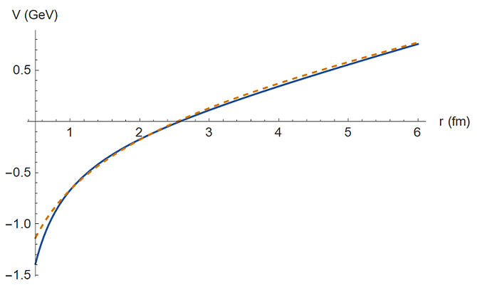
Figure 1 The Cornell potential [30] and the logarithm potential are plotted as a function of r. The blue line represents the Cornell potential and the dotted line represents the logarithm potential.
By presenting
We use the basic approximation to solve the previous equation analytically, taking into consideration that r < 1 fm. Function approximation
where
for which Eq. (7) becomes
where
Since Eq. (10) can be solved analytically.
Where
where
then we get,
The mass equation is found by solving Eqs. (15)-(17) with Eq. (11).
where
The diquark masses are calculated using Eqs. (18) and (19), as shown in Table II.
3. Numerical results and discussion
The mechanism underlying unusual state binding is currently unknown. The following three types of models can be used to ascribe various interpretations. (i) The molecular model of mesons and baryons, or their mixing. A chiral effective Lagrangian technique, the color-screen model, the QCD sum rules, and the scattering amplitudes approach were used to estimate the energy spectrum for this model. (ii) Diquark (triquark) interaction models, including compact diquark-triquark model and the diquark-diquark-antiquark model. As a result, the diquark-triquark model, as described in Ref. [38], is possible. In addition, as shown in Refs. [39,40], a classification of all possible pentaquark states
Only diquarks in the ground state N2S+1 LJ = 13 S1 are considered, and the diquark total spin must be 1 to preserve the Pauli exclusion principle. As a result, the diquark's total wave function will be anti-symmetric. These are known as axial-vector diquarks, and Jaffe [41] called these excellent diquarks.
In Table II, we noted that the diquark was slightly greater than the sum of its constituent quarks. Since we deal with diquark (quark-quark) as a bound state which required the binding energy to build them which gives by E = M - m1 - m2. They differ by no more than 200 MeV from the values for the diquark masses given in Table II and are actually in good accord with the findings in Refs. [32,34,37], which is proposed in the framework of non-relativistic quark systems. The Bethe-Salpeter and the Schwinger-Dyson equations, which take into account kinetic energy and also splittings in the spin-orbit, spin-spin, and tensor interactions, are used to study the diquark masses in Ref. [35]. Their diquark masses are estimated to be about 300 MeV higher than ours. Relativistic models based on QCD sum rules, as those in Ref. [36], projected smaller diquark masses. (With the cc diquark mass excluded, this indicates a higher mass).
In Table III, the tetraquark ground state mass spectrum is shown. Overall, lighter tetraquarks have a greater range of energy eigenvalues than heavier ones, resulting in a greater relative difference in mass between states for lighter tetraquarks compared to heavier ones. We analyze systems with the use of the various parameters of principal quantum number, orbital angular momentum, spin, and total angular momentum. Tetraquarks with total spins of 0, 1, and 2 are produced using a combination of spins, spin 1 diquark, and spin 1 antidiquark. In this non-relativistic method, quantum mechanic couplings were introduced, where the orbital angular momentum LJ couple into total angular momentum JT and total spin S.
Table III The masses of tetraquark in N2S+1 LJ (in GeV).
| Tetraquark | N2S+1 LJ | M(our) |
|---|---|---|
|
|
11 S0 | 4.049 |
| 13 S1 | 4.053 | |
| 15 S2 | 4.069 | |
| 11 P0 | 4.213 | |
| 13 P1 | 4.370 | |
| 15 P2 | 4.441 | |
| 11D0 | 4.675 | |
| 13D1 | 4.91 | |
| 15 D2 | 5.03 | |
|
|
11 S0 | 6.609 |
| 13 S1 | 6.611 | |
| 15 S2 | 6.629 | |
| 11 P0 | 6.531 | |
| 13 P1 | 6.611 | |
| 15 P2 | 7.034 | |
| 11D0 | 6.464 | |
| 13D1 | 6.52 | |
| 15 D2 | 7.22 | |
|
|
11 S0 | 11.0164 |
| 13 S1 | 11.032 | |
| 15 S2 | 11.049 | |
| 11 P0 | 11.013 | |
| 13 P1 | 11.061 | |
| 15 P2 | 11.173 | |
| 11D0 | 11.009 | |
| 13D1 | 11.05 | |
| 15 D2 | 11.23 | |
|
|
11 S0 | 20.012 |
| 13 S1 | 20.016 | |
| 15 S2 | 20.028 | |
| 11 P0 | 20.01116 | |
| 13 P1 | 20.0162 | |
| 15 P2 | 20.078 | |
| 11D0 | 20.013 | |
| 13D1 | 20.017 | |
| 15 D2 | 20.104 |
Table IV, shows our projected values for tetraquark masses as well as those from other studies. The results reported in Refs. [42,43] for
Table IV Comparison of tetraquarks masses (in GeV) in the ground state N2S+1 LJ with other works.
| Tetraquark | N2S+1l | M (our) | Ref. [32] | Ref. [42] | Ref. [43] | Ref. [34] | Ref. [44] | Ref. [45] |
|---|---|---|---|---|---|---|---|---|
|
|
11 S0 | 4.0497 | 4.076 | 3.849 | 3.852 | — | — | — |
| 13 S1 | 4.053 | 4.156 | 3.822 | 3.890 | — | — | — | |
| 15 S2 | 4.069 | 4.262 | 3.946 | 3.968 | — | — | — | |
|
|
11 S0 | 6.609 | 6.198 | — | — | 6.322 | 6.487 | 7.016 |
| 13 S1 | 6.611 | 6.246 | — | — | 6.354 | 6.50 | 6.899 | |
| 15 S2 | 6.629 | 6.323 | — | — | 6.385 | 6.524 | 6.956 | |
|
|
11 S0 | 11.0164 | 10.445 | — | 10.473 | — | — | — |
| 13 S1 | 11.032 | 10.472 | — | 10.494 | — | — | — | |
| 15 S2 | 11.049 | 10.523 | — | 10.534 | — | — | — | |
|
|
11 S0 | 20.012 | 18.754 | — | — | 19.666 | 19.322 | 20.275 |
| 13 S1 | 20.016 | 18.768 | — | — | 19.673 | 19.329 | 20.212 | |
| 15 S2 | 20.028 | 18.797 | — | — | 19.68 | 19.341 | 20.243 |
4. Conclusion
The non-relativistic Bethe-Salpeter equation is used to describe a tetraquark with two heavy-valence quarks by the current potential, that contains the logarithmic, linear and harmonic potentials and spin-spin interaction. The approach includes computing diquark masses from single quark interactions, then computing the four-quark state mass formed by one diquark and one antidiquark, which results in the tetraquark as shown in Fig. 2. Results in the literature that accurately characterize tetraquarks were compared to our findings and found to be in good agreement. Our results of the heavy tetraquark may be useful for future experimental data.
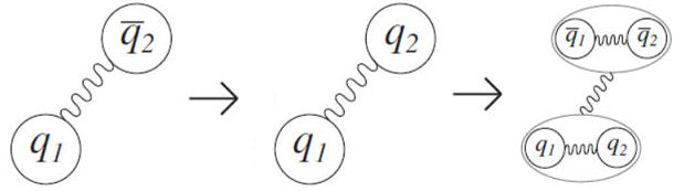
Figure 2 A diagram illustrating the modelling process. First, take the

