


 text new page (beta)
 English (pdf)
 Article in xml format
 Article references
 Send this article by e-mail
 Cited by SciELO
  Similars in
SciELO
Similars in
SciELO 
 Permalink
1. Introduction
Today it is possible to get laser pulses of high intensities even to relativistic orders, with their duration lasting less than a femtosecond. That is why studying the tunneling ionization process, which occurs when a laser interacts with matter, is much easier. This analysis was impossible before the 1980s. Experimental confirmation of the existence of this process1 opened a completely new chapter in quantum physics. It enabled the approach to many important scientific issues from a totally different perspective, such as radioactive decay2,3, the scanning tunneling microscope (STM) that gives information about surface topography6-8; in the area of public health and safety, as an innovative concept for nanostructure-based gas ionization sensors ; a technique called “tunneling ionization with a perturbation for the time-domain observation of an electric field” (TIPTOE) was developed. Using TIPTOE, the temporal profile of an input pulse can be determined by modulation of the ionization yield using an appropriate reconstruction algorithm9-10.
In a well-defined combination of strong intensity and a correspondingly low frequency of the laser field, in the infrared or optical domain, electron tunneling occurs through a potential barrier, which is impenetrable in classical mechanics. The laser electric field suppresses the Coulomb potential and thus forms a barrier through which the electron can tunnel. To describe the tunneling process, scientists have developed models and theories. Just a few of them will be mentioned. Starting from the Schrödinger equation for a hydrogen atom in a uniform electric field, Landau and Lifshitz determined the ionization probability (per unit of time)11. In 1965. Keldysh wrote a paper whose essence was to express rate as a sum of multiphoton processes, given as a total ionization rate12. He derived a relatively complex formula, but using the function:
The resulting formula given by the ADK theory describes the tunnelling process in which an unstable system decays according to the exponential law. The probability of survival of such a system decreases exponentially with time t. This method of calculating the tunnel ionization rate has become accepted and widely used, but tunneling can also be analyzed in a non-exponential mode17,18. To mention briefly, in the 1920s, the law of decay in the exponential form was established19,20. In the 1950s Khalfin21 assumed the existence of decay, which can be described by a non-exponential law, and his assumptions were proved experimentally22,23. Time dependence of non-exponential decay is in the form t-3/2, but Nicolaides and Beck24 suggested in their paper that this dependence could be ∼t-1. For non-exponential decay in a many-particle system that takes place over a longer period. This dependence is also possible in the form t-N , where the quantity N is proportional to the number of particles and depends on the quantum Bose-Einstein or Fermi-Dirac statistics of these particles. There are several approaches how to determine the tunneling time. One of them is Keldysh’s12, in which tunneling through a barrier is instantaneous and doesn’t take a finite time. Buttiker and Landauer considered time to be imaginary because it is thought that a breakdown of a wave function is below the barrier25. One of the concepts is that the tunneling time is viewed as an average value, not as a quantity that is strictly determined. Using this way of approaching the problem, the Feynman path integral (FPI) was obtained26,27, which can be presented as a process of averaging using the tunneling time of probability amplitude. The development of science enables us to solve this dilemma experimentally. Now it is possible to determine the real tunneling time using attoclock measurements in a wider range of laser field intensities28. For a more detailed analysis of the tunnel ionization process and calculation of the ionization probability distribution of ejected electrons, it’s important to take into account the spatial distribution of a laser beam profile when optimizing the experimental setup. Laser systems can operate with near-Gaussian beams or non-Gaussian beams. The most commonly used models of laser beam shaped profiles, in physics as well as in other branches of sciences, are Gaussian29,30, Super-Gaussian (SG) (flat-top beams where a beam exhibits a nearly constant irradiance over its beam width)31, Hermite-Gaussian (HG) (rectangular)32-34, cylindrical and are called Laguerre-Gaussian (LG)35,36, as well as Lorentzian37. Experimentally it is possible to achieve a transition from a spot-like profile of the laser beam to a doughnut shape, and vice versa38-40. The processes that take place under the influence of the laser field must be discussed theoretically by including different spatial distributions of the laser beam, from fundamental modes (Lorentzian and Gaussian) to higher-order beam modes (SG, HG, LG). This paper report results obtained by calculating and estimating the effects of different laser beam profiles on ionization probability distributions in a wide range of laser intensities for the specific wavelength in the infrared domain, when the electron tunneling time is in the range of t = (1 - 800) as. Potassium was chosen as the target atom exposed in a linearly polarized laser field. This model is applicable in a non-relativistic regime, for laser intensities less than 1018 W/cm2. It could be extended to a relativistic regime for much higher intensities, with the inclusion of required relativistic corrections, but this would be out of the scope of this paper. Research in the fields of ultrahigh laser intensities exceeding 1020 W/cm2 would allow studying multiple tunneling ionization of heavy atoms41,42.
The structure of our paper is the following. After the introduction, the theoretical background is presented in Sec. 2, followed by a presentation of the results and discussion (Sec. 3) where the probability distribution in exponential and non-exponential modes was calculated. In Sec. 4 we gave our conclusions. A complete description of the systems of probability equations, as well as all the parameters needed for their implementation, are given in atomic units (|e| = me = ħ = 1).
2. Theoretical background
An unstable system has multiple ways of decaying: spontaneous decay, tunneling alpha decay of atomic nuclei, single-photon ionization of atoms, etc. The basic formulas used to describe each of the decay processes are43:
where |S〉 is the state vector, H is the Hamiltonian of an unstable system, while a(t) and P(t) is the decay survival probability amplitude and the survival probability, respectively. The unstable state |S〉 is not an eigenstate of the Hamiltonian H, and the energy distribution of this state can be defined as:
where the energy normalization condition holds:
In order to discuss the probability distribution of exponential and non-exponential tunneling ionization of atoms exposed to an intense laser field, it is necessary to define the probability amplitude for both of these mechanisms.
2.1. Exponential decay
The energy distribution of an ejected electron of the exponential decay, with respect to mean electron energy ϵ, is given by the Breit-Wigner distribution44:
where Γ(E) is the decay width. A detailed derivation of this equation can be found in Ref.45. The first step in deriving the probability amplitude is to apply the Fourier transform using a complex integral:
Function F(w) has two simple poles at w = ∈ ± i(Γ(∈)/2). The integral at pole w = ∈ + i(Γ(∈)/2) diverges and correspond to an unphysical state; therefore we account only for the contribution from the simple pole located at w = ∈ - i(Γ(∈)/2) in order to obtain an exponentially decaying state.
By the residue theorem:
The first integral tends to zero,
The notation arc means arc length and represents the distance between two points along a section of a curve. Eq. (5) can be written in the following form:
by applying the residual theorem Eq. (7) and after several mathematical transformations the Breit-Wigner probability amplitude can be obtained:
A suitable simple pole at E = ∈ - i(Γ(∈)/2) in Eq. (9) provides:
which leads to the formula for the probability amplitude of the initial state:
The decay width Γ = 1/τ is the inverse of a lifetime, which is the initial decay rate, and can be measured by fitting the counting rate of decay products to the exponential law:
where dN(t) is the number of decay products registered in the detector during the time interval dt. In the case of the tunneling ionization of an atom in a strong low-frequency laser field the width Γ(E) can be represented by the equation18:
where E is the kinetic energy and has values greater than zero, E > 0. The probability amplitude is interpreted as the possibility of the appearance of a particle (in our case an electron) at the moment 𝑡 when it’s mean kinetic energy is ∈. The probability amplitudes are complex numbers. The corresponding probability is proportional to the modulus squared of the probability amplitude, which, unlike the amplitude, is a positive real number. The square of the module of Eq. (11) gives:
where the mean electron energy E = ∈ corresponds to the average kinetic energy of the ejected electron that oscillates in the electric field and it is equal to the ponderomotive potential. The ponderomotive potential for a linearly polarized laser field has the form ∈ = Up = F2/(4(2). Using the expression for mean electron energy ∈ and substituting expression Eq. (13) into Eq. (14) probability is defined as:
where is
2.2. Non-exponential decay
To get a basic insight into the mechanism of non-exponential ionization of the tunnel, it is required to calculate the appropriate probability amplitude as a function of time. Starting from Eqs. (5) and (7) the following is obtained48:
Choosing a negative imaginary axis is useful for calculating a long time limit. The analysis will remain unchanged when using this integration contour, as long as the contour closes the physically relevant poles near the positive real axis. After implementing the replacement y = xt, the equation above becomes:
Knowing that at t → ∞ the non-exponential decay is determined by small values of E → ∞, the denominator in ([eq:non_exp_probability_amlitude_2]) becomes equal to ∈2:
This time limit determines the behavior of near zero, that Γ(-y/t) = Γ(0)48,49:
In accordance with Eq. (13), the non-exponential decay width is obtained:
This derivation leads to a finite expression for probability in a non-exponential mode:
In the tunnel ionization regime, the total probability can be viewed as a function of P(F, t), which maps values into real numbers over the range of [0,1]. A detailed theoretical analysis of the ionization probability gives us an advantage in better understanding of the experimental data. Experimental determination of absolute ionization probabilities is complicated because ionization of atoms in strong laser fields depends on various experimental setups: target density, excited state fraction, incoming photon flux, detector efficiency and relative spatial alignment of the target and laser pulse50,51. Therefore, we tested the influence of different beam profiles on exponential and non-exponential probability distributions. The Gaussian (G) beam profile was the first we paid attention to. The electric field for this beam profile can be expressed as30,31:
where r2 is the distance from the centre of the beam,
n represents the order/index of the Super-Gaussian beam, and it’s value is n > 2. The case n = 2 corresponds to the basic Gaussian profile. It is shown that the Super-Gaussian beam of the higher index and smaller beam width can produce much stronger radiation compared to the Gaussian beam52. By differentiating the fundamental Gaussian mode, higher-order beams like Hermite-Gaussian and Laguerre-Gaussian with complex arguments can be obtained. These calculations can be generalized to deriving a whole family of Hermite-Gaussian (HG) and Laguerre-Gaussian (LG) modes, including also those with real arguments53,54. Field intensity distributions of higher-order HG mode laser beams and the amplitude of the electric field are given in literature55,56. For this research the Hermite-Gaussian beam of the first order was used:
The Hermite-Gaussian mode is closely related to the Laguerre-Gaussian mode, and some research requires conversion of the HG into the LG mode and vice versa. The way this can be performed is given in literature57. The behavior of tunneling probabilities under the influence of a LG(0,1)* spiral phase mode was also analyzed. The electric field for a linearly polarized laser light with this beam profile is given by58:
where ra(𝜙) = aeκa 𝜙 is the polar equation, a and ka are constants, while 𝜙 is the azimuthal angle. More about LG beams can be seen in Refs.59-61. In experiments, high laser intensities are involved. It has been shown that the transverse intensity profile is not always described well by a Gaussian distribution62,63 and that Lorentzian’s (L) distribution would be more appropriate40,64,65. A Lorentzian electric field distribution function was propounded in work of Shealy et al.66:
Experiments in the attosecond domain indicated that the tunneling time is much shorter than predicted by theories67,68. The presented laser beam profiles in combination with controlled light pulses lasting attoseconds (10-18s), made it possible to observe what happens during ionization, providing the possibility of a detailed analysis of the process.
3. Results and discussion
The behavior of an atom located in the external electromagnetic field, directed along the z axis, can be conveniently investigated in parabolic coordinates: ξ = r + z, η = r - z, 𝜙 = arctan (y/z), where 𝜙 is the azimuthal angle, 𝜙 ∈ [0, 2(], ξ, η, ∈ [0, ∞). Conversely in Cartesian coordinates
The potential barrier through which the electron tunnels is along the η coordinate in the direction z → -∞, where the η coordinate has higher values. The exit point is determined by ηexit ≅ 1/F in the range 1 << η << ηexit.11,69 The laser field strength for linearly polarized light in atomic units is approximately equal to ∼5.4 x 10⁻⁹ √I, and within a broad intensity range (1012 - 1015) W/cm2, exponential and non-exponential tunneling was observed. These intensities correspond to the values of ( coordinates in the range 6 - 185 a.u.. The investigation was performed when the exit point was η = 10. It is possible that the tunnel exit point is located in this region for the laser intensity I ∼3 x 10¹⁴ W/cm2. Calculations were done for an intense infrared Ti: sapphire laser pulse with wavelength λ = 800 nm (15117.2 a.u.), beam waist of w0 = 4 mm (7.559 ( 107 a.u.)70,71 and photon energy w = 0.05696 a.u. It should be emphasized that the beam waist can be in a wide range of values, from micrometers (3 - 60) (m to millimeters (15 - 30) mm. Higher-order beam modes correspond to the narrower beam waist and w0 has to be adapted. The target to which this beam is directed is the potassium atom with the ionization potential of valence electron of Ip = 4.3406 eV (0.1595 a.u.). The value of the Keldysh parameter is y = 0.1, which is in the range of values given by the condition y << 1 that defines the domain of tunnel ionization.
To calculate the probability for a Laguerre-Gaussian beam shape, it was necessary to define the values of the parameters that appear in Eq. (26).
3.1. Exponential mode
The exponential probability distribution is given Eq. (15) when a field strength of a laser pulse is approximately equal to the root of the field intensity and without a defined spatial distribution (F ∼ √I), hereinafter referred to as basic. The behavior of the probability distribution is observed in a wide range of laser field intensity and tunneling time interval (1 - 800) as, which is sufficiently long enough for an ionization event to occur (as confirmed in experiments28,73). It should be emphasized that the Figures given in the text are computed for laser intensity in the interval (1012 - 5 ( 1015) W/cm2. However, in the laser intensity range of (1012 - 1013) W/cm2 the probability is negligible, so in Figs. 1-10 we showed the probability distribution for the laser intensity range of (1014 - 1015) W/cm2.
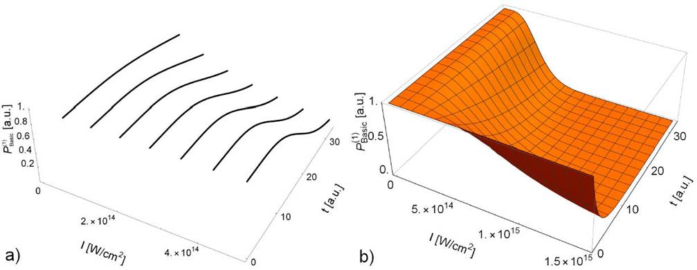
Figure 1 Exponential probability distribution P(1)Basic for the tunneling time range t = (1 - 800) as i.e. t = (0.041 - 33.073) a:u: (a) in the interval of laser intensities I = (1014 - 5 ( 1014)W/cm2, (b) I = (1014 - 1.5 ( 1015) W=cm2.
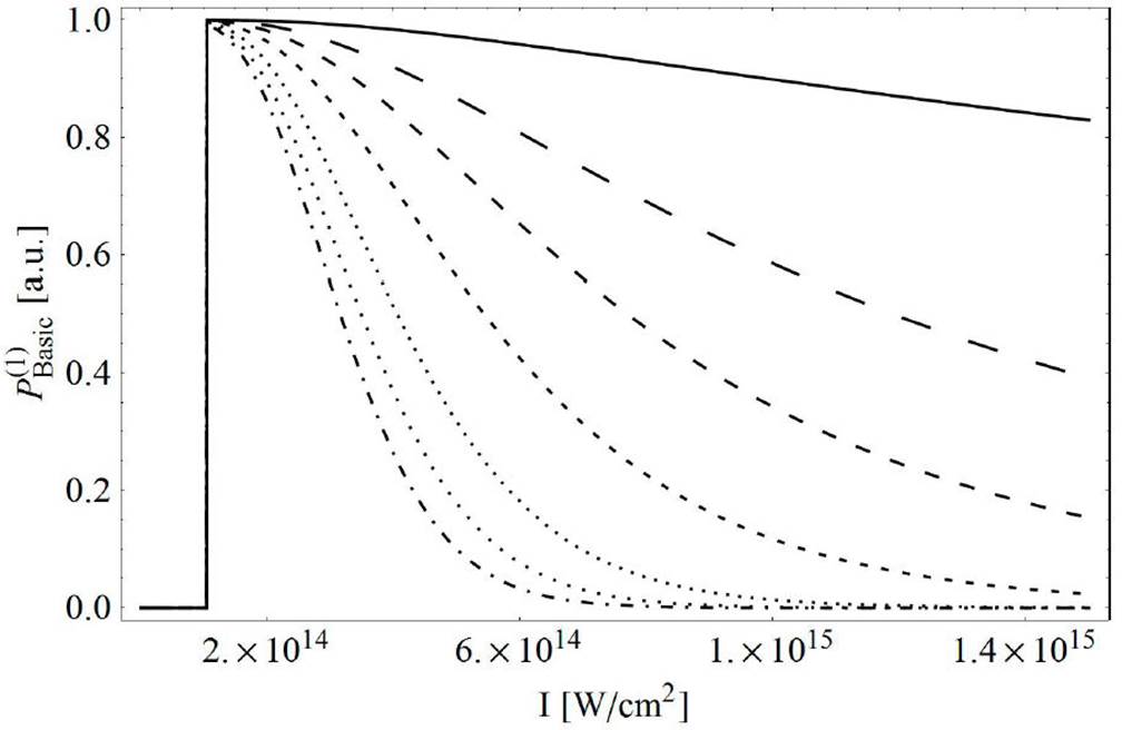
Figure 2 Exponential probability distribution P(1)Basic, for the laser intensity range I = (1014 - 1.5 ( 1014) W/cm2. Each probability curve corresponds to an integer value of attoseconds of tunneling time t1 = 1 as (solid line), t2 = 50 as (large dashed line), t3 = 100 as (medium dashed line), t4 = 200 as (small dashed line), t5 = 400 as (tiny dashed line), t6 = 600 as (dotted line), t7 = 800 as (dot-dashed line).
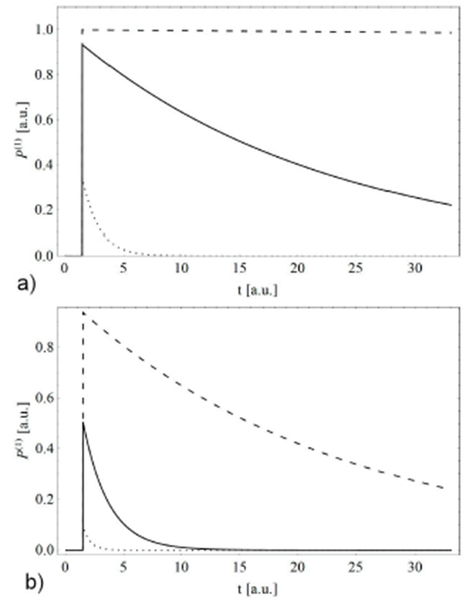
Figure 3 Exponential probability distribution as a function of the tunneling time. P(1)G, P(1)SG (beam order n = 4), P(1)L, (solid line), P(1)HG (dotted line), P(1)LG(SP)(dashed line). Tunneling time is in range of t = (1 - 800) as with corresponding value in atomic units t = (0:041-33.073)a:u: laser intensity is fixed a) at I = 4.2 x 10¹⁴ W/cm2, b) at I = 1.5 x 10¹⁵ W/cm2.
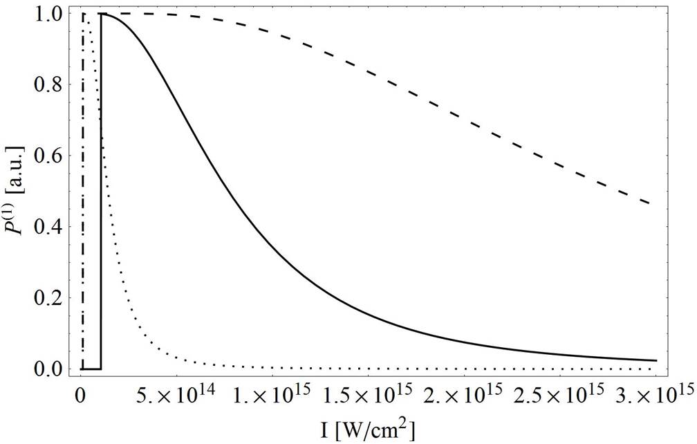
Figure 4 Exponential probability distributions. P(1)G, P(1)SG(beam order n = 4), P(1)L (solid line), P(1)HG (dotted line), P(1)LG(SP)(dashed line) vs laser intensity in range I = (1014 - 3 x 10¹⁵) W/cm2 for fixed value of tunneling time t = 100 as (4.13 a:u:).
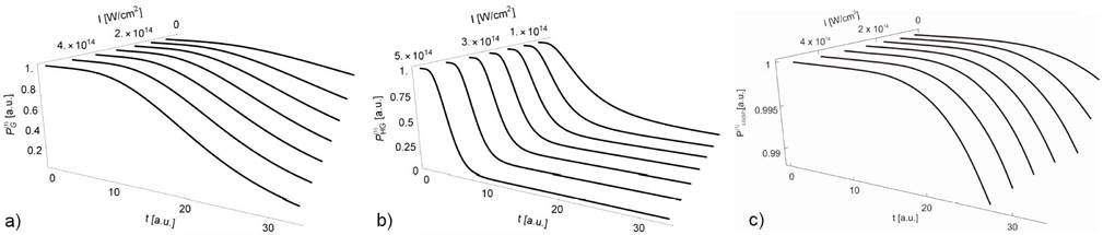
Figure 5 Exponential probability distributions P(1)G, P(1)HG, P(1)LG(SP) 2D curves plotted into the 3D coordinate system for the intensity range I = (1014 - 5 x 10¹⁴) W/cm2 and tunneling time t = (1 - 800) as.
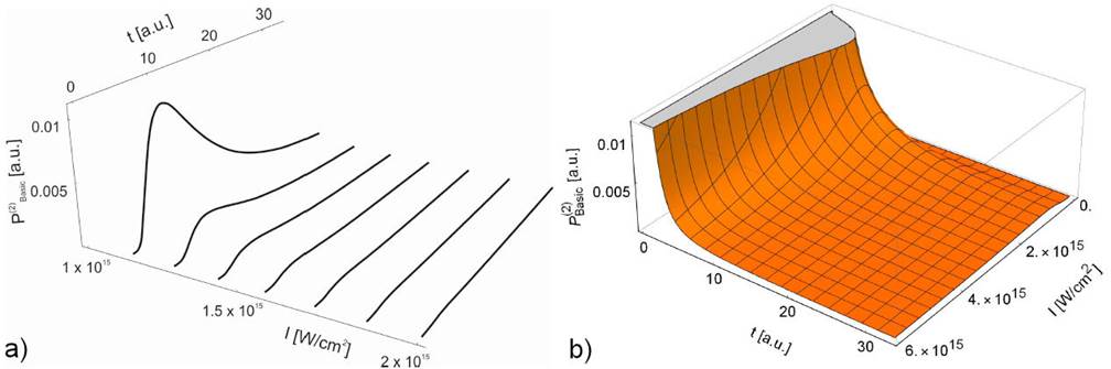
Figure 6 Non-exponential probability distribution P(2)Basic, as a function of tunneling time in the interval t = (1 - 800) as and laser intensity range: a) I = (1015 - 2 x 10¹⁵) W/cm2, b) I = (1015 - 6 x 10¹⁵) W/cm2.
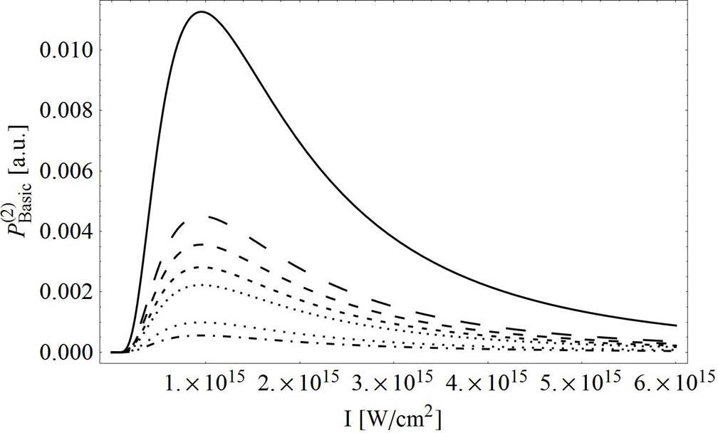
Figure 7 Non-exponential probability distribution P(2)Basic, for the laser intensity range I = (8 x 10¹⁴ - 6 x 10¹⁵) W/cm2. Each probability curve corresponds to an integer value of attoseconds of tunneling time. t1 = 1as (solid line), t2 = 50as (large dashed line), t3 = 100 as (medium dashed line), t4 = 200 as (small dashed line), t5 = 400 as (tiny dashed line), t6 = 600 as (dotte line), t7 = 800 as (dot-dashed line).
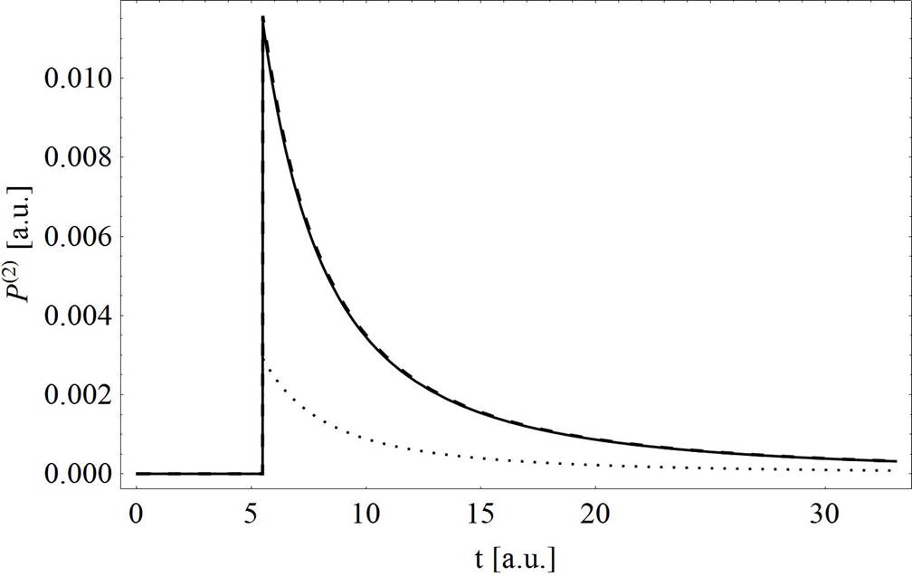
Figure 8 Non-exponential probability distribution P(2) G , P(2)SG (beam order n = 4), P(2)L (solid line), P(2)HG (dotted line), P(2)LG(SP) (dashed line) as a function of tunneling time in range of t = (1 - 800) as for fixed value of laser intensity at I = 1.2 ( 1015 W=cm2.
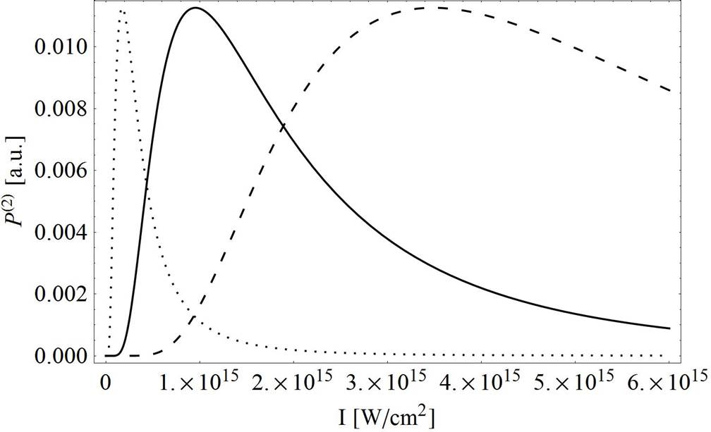
Figure 9 Non-exponential probability P(2)G, P(2)SG (beam order n = 4.), P(2)L (solid line), P(2)HG (dotted line), P(2) LG(SP) (dashed line) vs laser intensity in range I = (8(1014-6(1015) W=cm2 for fixed value of tunneling time t = 1 as (0.0413411 a:u:).
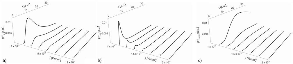
Figure 10 Non-exponential probability distributions P(2)G , P(2)HG, P(2)LG(SP) 2D curves plotted into a 3D coordinate system for intensity range I = (1015 - 2 ( 1015) W/cm2 and tunneling time t = (1 - 800) as.
P(1)Basic 2D curves, plotted into a 3D coordinate system, provide the opportunity to quite clearly notice the dependence of the exponential probability distribution on the tunneling time for the specific values of the laser field intensities: (0.8x10¹³, 1.4x10¹⁴, 2.0x10¹⁴, 2.6x10¹⁴, 3.2x10¹⁴, 3.8x10¹⁴, 4.4x10¹⁴) W/cm2, (Fig. 1a). At the field intensity of (1014 W/cm2, no matter how long the tunneling time is, the distribution of the electron ionization probability changes very little, while with increasing field intensity, the maximum probabilities are more pronounced. It can be assumed that an electron in a very short time interval receives an amount of energy sufficient to pass through a potential barrier so that the tunneling time with increasing intensity becomes shorter.
Dependences of the ionization process for any values of tunneling time in an extended range of intensities I = (1012 - 1.5 x 10¹⁵) W/cm2 can be estimated from the 3D surface (Fig. 1b). In very intensive fields, the exponential probability distribution of the tunneling time reaches a maximum for t ∼1 as. As the laser field intensity increases, the range of values of the tunneling time narrows. The probability distribution P(1)Basic as a function of laser field intensity for the fixed integer value of attosecond tunneling time is shown in Fig. 2. The probability sharply increases with the increase of laser intensity for all observed tunneling time values, then reaches a maximum at the same field intensity 0.2x10¹⁴ W/cm2 and then with a further increase of intensity decreases slightly in different ways. The longer the expected tunneling time is, the faster the probability decreases.
For the tunneling time of 1as (0.041 a.u.), a maximum probability value is P(1)Basic = 1 or P(1)Basic ≈ 1 for almost all the field intensities ranges. With the tunneling time increase up to several hundred attoseconds and with increasing laser intensity, the probability decreases, which corresponds to the physical picture that the electron requires real time to tunnel through the barrier, in fact, as the interaction time with the electron shortens, the probability that the electron will completely tunnel through the barrier becomes greater74. The probability reaches a maximum at a precisely defined laser intensity and then decreases monotonically, which is the effect of atom stabilization in the superintense field75.
By including Eqs. (23), (24), and Eq. (27) in Eq. (15) we obtained probability distributions
For the tunneling time t = 100 as the probability distribution
Tunneling time duration intervals differ from profile to profile of the laser beam (5). The shortest time interval gives the HG beam profile and
3.2. Non-exponential mode
In order to get a basic insight into the tunnel ionization process in a non-exponential regime, calculations analogous to the previous analysis were performed. For inception, the non-exponential probability distribution (Eq. (22)) for the basic form of laser field distribution was calculated. In contrast to the exponential mode, the maximum probability distribution reached much lower values at higher laser intensities. In 6a the ionization probability distribution P(2)Basic 2D curves plotted into a 3D coordinate system is obtained as a function of the tunneling time (t = (1- 800) as) and concrete values of laser intensities: (4.0(1014, 7.0(1014, 9.0(1014, 1.3(1015, 1.5(1015, 1.75(1015, 2.0(1015) W/cm2. It can clearly be seen that the position of the peak does not change, but reached maximum values decrease with increasing field values. The tunneling time interval narrows from t = (1- 500) as to instantaneous tunneling at higher laser intensities. The laser field is stronger so the potential barrier is suppressed and the electron needs a shorter time to pass through. Using the 3D surface plotting method, in a wide range of laser field intensity and full interval of tunneling time, a more complete picture of the ionization probability P(2)Basic behavior is obtained. A steep drop with a long plateau was observed (Fig. 6b).
Assuming how long the tunneling time can last, the probability distribution dependence on the intensity of the laser field was analyzed Fig. 7. As the tunneling time increases, the non-exponential probability distribution decreases. The maxima shift to the left, towards lower intensities, which corresponds to a larger barrier width.
We have computed the probability distributions by combining Eqs. (23-27), with Eq. (22) and present them in Fig. 8. It is shown that P(2)Non-exponential is completely independent of most laser beam profiles. For a fixed laser intensity 1.2(1015 W/cm2, all probability distributions overlapped perfectly except P(2)HG. The P(2)HG probability distribution has a five times lower value and a much narrower time interval in which tunneling is possible. P(2)G, P(2)SG, and P(2)L non-exponential probability distributions reached maximums at a stronger field intensity, compared to the exponential mode, 0.95(1015 W/cm2 (Fig. 9). The positions of maximums define the exit point of the barrier, so it can be seen that this point will be shifted using LG and HG laser beam profiles. The resulting peaks appear at 3.4(1015 W/cm2 and 1.6(1014 W/cm2 intensities of the laser field for P(2)LG(SP) and P(2)HG, respectively (Fig. 9).
Variations of the non-exponential probability distribution for the corresponding laser beam profiles, computed following the numerical procedure outlined above, are shown in Fig. 10. In a broad range of tunneling time, P(2)G, P(2)HG, P(2)LG(SP) probabilities behave similarly, reach a maximum and then decrease with a long asymmetric tail appearing. Along with an increase of tunneling time, the position of the probability peaks changes. With increasing laser intensity, the maximum values of probabilities become smaller, and at certain field intensities, they are so small that they approach zero.
The analysis is extended into the region of the entire infrared spectrum. Figure 11 presents the results of comparison of the non-exponential probability distribution surfaces P(2)G, P(2)LG(SP), P(2)HG, for a fixed laser intensity 1.3(1015 W/cm2. It is observed that the tunnel ionization in the non-exponential domain for these laser beam shapes becomes possible in the region w > 0.04 a.u. which corresponds to λ > 1.138 (m.
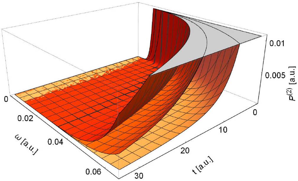
Figure 11 Non-exponential probability distributions P(2)G (red), P(2)LG(SP) (orange), P(2)HG (light orange) vs tunneling time in the interval t = (1 - 800) as and photon energy ! = (0.0000456 - 0.0651) a:u: which corresponds to the entire infrared spectra λ = (700 x 10-9 - 1 x 10⁻³) m. Laser intensity is fixed at I = 1.3 ( 1015 W/cm2.
4. Conclusion
Our paper reported calculation and analysis of the probability distribution of exponential and non-exponential tunneling ionization for the valence electron of a potassium atom exposed to a linearly polarized strong laser field using a broad range of laser intensities. This discussion is presented to investigate the effects of different laser beam profiles that propagate differently and exhibit significantly different spatial distributions on the ionization probability distribution in both modes. Several laser beam profiles were used: fundamental Gaussian and Lorentzian (low-order beams) and Super-Gaussian, Laguerre-Gaussian and Hermite-Gaussian (high-order beams). It was found that application of Gaussian, Lorentzian and Super-Gaussian beam profiles does not affect the exponential probability distribution. Moreover, appropriate probabilities matched perfectly and gave the same tunneling time interval on any laser intensity in the observed range. In the case of Laguerre-Gaussian and Hermite-Gaussian beam profiles, the tunneling time interval is completely different. The probability distribution for the LG profile has a maximum in a large range of tunneling times. On the other hand, the HG probability, for the same parameters, has lower values while the tunneling time is in a much narrower range. Calculations in the non-exponential mode showed that the probability distributions reached a hundred times lower maximum values at much higher laser intensities than in the exponential mode. In the non-exponential mode, all beam profiles give a broad interval of tunneling time, except in the Hermite-Gaussian case where this interval is constricted. In the region of the infrared spectrum, where w > 0.04 a.u. (λ > 1.138 (m), non-exponential probability distributions are approximately equal to zero. Non-exponential ionization becomes possible only at higher frequencies. The results presented above indicate that the difference between probabilities, computed for lower and higher-order beam field distributions, could be associated with spatial propagation characteristics of the higher-order beam. The spatial beam pattern of the higher-order modes is preserved during propagation to increase the slope of the spatial electric field at any position along the path.

