SciELO - Scientific Electronic Library Online

 
vol.12 número3Relationship between age-sex classes and prevalence of Giardia spp. and Blastocistys spp. in black and gold howler monkeys inhabiting fragmented forestsEthological studies of native Mexican mammals: A review índice de autoresíndice de assuntospesquisa de artigos
Home Pagelista alfabética de periódicos  

Serviços Personalizados

Journal

Artigo

Indicadores

Links relacionados

  • Não possue artigos similaresSimilares em SciELO

Compartilhar


Therya

versão On-line ISSN 2007-3364

Therya vol.12 no.3 La Paz Set. 2021  Epub 28-Mar-2022

https://doi.org/10.12933/therya-21-1088 

Articles

Use of distribution models in the conservation of a Mexican endemic lagomorph

Luis José Aguirre-López1  * 

Tania Escalante1 

1Grupo de Biogeografía de la Conservación, Departamento de Biología Evolutiva, Universidad Nacional Autónoma de México, Facultad de Ciencias. Circuito interior s/n, Coyoacán, C.P. 04510 Ciudad Universitaria, Ciudad de México, México. Email: luisjose@ciencias.unam.mx (LJA-L), tescalante@ciencias.unam.mx (TE).


Abstract:

The volcano rabbit (Romerolagus diazi), endemic to the central-eastern Transmexican Volcanic Belt, is one of the most threatened lagomorphs worldwide. Several factors threaten to decrease its geographical distribution, which is already restricted to the Pelado, Tláloc, Iztaccíhuatl, and Popocatépetl volcanoes. Our study aimed to propose priority areas for the conservation of this rabbit within Iztaccíhuatl-Popocatépetl National Park (IPNP) based on species distribution models. Volcano rabbit presence data were collected through different field sampling techniques and public and private databases. The environmental predictors used to model suitability were obtained from both open-access remote sensors and topographic information. The models’ performance was adjusted by evaluating different sets of variables and data to improve the certainty of the results. We obtained an area of 132.5 km2 within the IPNP potentially occupied by the volcano rabbit and a high suitability area of 7 km2. In addition, four priority conservation polygons for the volcano rabbit were identified within the National Park. We showed that the suitability and potential distribution are not uniform in the park, being the alpine meadow dominated by Muhlenbergia sp., the most suitable area for R. diazi. Therefore, the conservation strategies should focus on preserving these meadows in the prioritized polygons, avoiding tourist and unskilled personnel’s access. This work represents a contribution to the conservation of the volcano rabbit and a theoretical and practical tool for use in the IPNP.

Keywords: Ecological niche modelling; MaxEnt; natural protected area; remote sensing; suitability; volcano rabbit

Resumen:

El conejo de los volcanes (Romerolagus diazi), endémico del centro-este de la Faja Volcánica Transmexicana, es uno de los lagomorfos más amenazados en todo el mundo. Muchos factores amenazan con disminuir su distribución geográfica, la cual ya está restringida a los volcanes Pelado, Tláloc, Iztaccíhuatl y Popocatépetl. El objetivo de nuestro estudio fue proponer áreas prioritarias para la conservación de este conejo en el Parque Nacional Iztaccíhuatl-Popocatépetl (PNIP), con base en modelos de distribución. Los datos de presencia del conejo de los volcanes fueron colectados a través de diferentes técnicas de muestreo en campo y bases de datos públicas y privadas. Los predictores ambientales usados para modelar idoneidad fueron obtenidos de sensores remotos e información topográfica, ambos de acceso libre. El desempeño de los modelos fue ajustado mediante la evaluación de diferentes conjuntos de variables y datos para mejor la certeza de los resultados. Se obtuvo un área de 132.5 km2 en el PNIP potencialmente ocupado por el conejo de los volcanes y un área de alta idoneidad de 7 km2. Además, se identificaron cuatro polígonos prioritarios para la conservación del conejo de los volcanes dentro del Parque Nacional. Aquí demostramos que la idoneidad y distribución potencial no son uniformes dentro del parque, siendo la pradera alpina dominada por Muhlenbergia sp., el área más idónea para R. diazi. Por lo tanto, las estrategias de conservación deberán enfocarse en preservar esas praderas en los polígonos priorizados, evitando el acceso de turistas y personal no calificado. Este trabajo representa una contribución a la conservación del conejo de los volcanes y una herramienta teórica y práctica para su uso en el PNIP.

Introduction

Romerolagus diazi (Ferrari-Pérez, 1893) is an endemic species of the central-eastern Trans-Mexican Volcanic Belt (TVB) biogeographic province (Barrera 1966; Velázquez et al. 1996), and it has been listed as endangered species with a decreasing estimated population of 7,000 individuals (Velázquez and Guerrero 2019). This rabbit is also known as the zacatuche, teporingo, or volcano rabbit; it is a monospecific and ancient genus with taxonomic, anatomic, and biogeographic features similar to Pentalagus and Pronolagus (Hoffman et al. 1994). The volcano rabbit is a gregarious species that form groups of two to five individuals, although the age and sex composition of these groups are unknown. To date, knowledge about home range or dispersal capacity is low (Rizo-Aguilar et al. 2014). However, Galindo-Leal and Velázquez (1996) suggested low dispersal capacity than other lagomorphs, and Cervantes and Martínez-Vázquez (1996) proposed a home range of 2,500 m2 based on their field research. In terms of reproduction, the gestation period is longer, and the litter size is smaller in these ancient rabbits compared to other rabbits (Cervantes 1982).

Romerolagus diazi faces intense human pressure due to agriculture expansion, poaching, and development for tourism and because its restricted distribution is surrounded by large cities, including Puebla, Toluca, and Mexico City. These situations modify, fragment, or destroy the specific habitat where R. diazi lives. All of these factors make this lagomorph species a priority conservation target. Also, its geographic distribution rarity increases its vulnerability (Lawler et al. 2003). If the species is extirpated from its known geographic distribution, there is no other place in the world to find it.

The Iztaccíhuatl-Popocatépetl National Park (IPNP) is located in the Mexican states of Puebla, México and Morelos (19.2362° N, -98.6634° W), and it has an area of 39,819 ha and a human population of 244 people (Instituto Nacional de Estadística y Geografía (INEGI 2010); Comisión Nacional de Áreas Naturales Protegidas (CONANP 2013); Secretaría de Medio Ambiente y Recursos Naturales (SEMARNAT 2013). A large part of the geographic distribution of R. diazi (Martínez-Meyer 2005; Farías et al. 2015) is located within the natural protected area of IPNP (Figure 1), which includes pine forest, alpine meadows, rocks without vegetation and the Popocatépetl volcano. In the IPNP, Osuna et al. (2020) identified two of the four linages of the teporingo, one at northern and the other at southern part.

The geographic distribution of a taxon depends on its ecological niche and dispersal ability (Soberón and Peterson 2005). Correlative methods link presence records of a taxon and its associated environmental variables, and therefore, they can be used to produce maps of potential distribution based on the theory of ecological niche (Soberón et al. 2017). In particular, species distribution models are representations in geographical space of the suitability of a place for a species’ presence, where suitability is the mathematical or statistical relationship between the actual distribution and a set of predictor variables (Mateo et al. 2011).

We aimed to prioritize zones with high suitability for the volcano rabbit within Iztaccíhuatl-Popocatépetl National Park (IPNP), using data derived from satellite and fieldwork, relating the utility of correlative methods with helpful conservation strategies.

Materials and Methods

Fieldwork. The fieldwork aimed to obtain georeferenced presence records of R. diazi. Our study area for fieldwork was located on the southern part of the IPNP between the Popocatépetl and Iztaccíhuatl volcanos, a 74 km2 site. Trap cameras were placed in the study area with a separation of 1 km between them. The cameras were installed 50 cm from the ground and were not impeded by vegetation. The cameras were operational from April 2018 through October 2018, with 2,138 camera days. Image processing was performed using Wild.ID 0.9.28 software (TEAM Network 2017). The following information was captured in the databases: project name, camera ID, geographic coordinates, date and time, type of photo, file name, taxonomic identification, number of animals, the person that identified, start date, end date, person who placed and removed the camera, camera model, and institution responsible. In addition to the camera images of volcano rabbits, their presence was recorded by direct and indirect observations. Throughout the study, transects were made to identify volcano rabbits and their latrines visually. The identification of latrines was based on a latrine surface area of approximately 20 cm x 20 cm, at least 20% fresh scat, a uniform discoid shape of feces, and a uniform 5 to 9 mm size of feces (Cervantes and Martínez-Vázquez 1996), with at least ten feces per latrine.

Data analysis. We performed different suitability models at a scale of 30 m to identify places with ideal conditions. To do this, we compiled the data obtained from our fieldwork into one database (model a) and in a separate database (model b) compiled data from fieldwork, GBIF data (biological collections or authors in Appendix 1), and data from the mammal database of the JM055 project funded by CONABIO (Escalante 2014). In both data sets, the locations were reviewed, and the points were filtered with a spatial resolution of 30 m. We used satellite images from November 7, 2017, January 10, 2018, and January 29, 2019, from Landsat 8 OLI/TIRS C1. United States Geological Survey (USGS 2019). First, we performed a radiometric calibration (conversion to reflectance with angular correction) of the Near Infrared (NIR), Red (R), and Shortwave Infrared 1 (SWIR1) bands (Ariza 2013; USGS 2013). Then, we used these calibrated bands to calculate the Normalized Difference Vegetation Index (NDVI; Rouse et al. 1973). To relate the NDVI values to specific vegetation types, six 50-m transects were performed in different areas and elevations of the IPNP. A 50-m rope was placed on the ground, and the vegetation under the rope was collected at one-m intervals. Plant species were identified ex-situ by César Miguel-Talonia (unpublished data). The NDVI values used for this vegetation characterization were from the satellite images from January 10, 2018, with the EPSG projection: 4326 - WGS84. The humidity was obtained using the Normalized Difference Moisture Index (NDMI; USGS 2013).

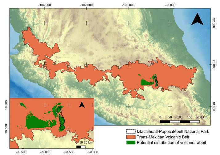
Figure 1 Iztaccíhuatl-Popocatépetl National Park is located at the center east of the Transmexican Volcanic Belt. The potential distribution for R. diazi (Farías et al. 2015) is shown in the lower-left corner into the IPNP. 

We estimated the surface temperature of the area using algorithms, as proposed by Wang et al. (2015) and Avdan and Jovanovska (2016). To do this, we first calculated the TOA (Top of Atmospheric Spectral Radiance; Barsi et al. 2014) from band 10 (TIR1) due to high uncertainty in the values of band 11 (TIR2; Wang et al. 2015). The value of O10 reported by Wang et al. (2015) is 0.29 (W·m−2·sr−1·μm−1), based on USGS files for dates before February 3, 2014. For later dates, as in our study, this value should not be included because the downloaded data is already processed, including this value (Wang et al. 2015). Secondly, we converted the reflectance to the brightness temperature (BT; USGS 2013), derived from an approximation of the Planck radiance function using the constants that appear in the product metadata. Third, we calculated the proportion of vegetation (Pv) from the range of NDVI (maximum and minimum) depending on the area (Carlson and Ripley 1997; Sobrino et al. 2004; Dash et al. 2005). Sobrino and Raissouni (2000) proposed values of NDVIS = 0.2 and NDVIV = 0.5 for global conditions. For particular areas, NDVIS and NDVIV can be extracted from the NDVI histogram (Sobrino et al. 2008). Next, we calculated the emissivity of the Earth’s surface (LSE, Land Surface Emissivity). In the wavelength range of Landsat 8 band 10, the emissivity can be calculated using the simplified threshold method for the NDVI (SNDVITHM; Sobrino et al. 2008). To calculate the emissivity, we used the values for general conditions proposed by Sobrino and Raissouni (2000). For NDVI values less than 0, the emissivity was assigned a value of 0.991; for NDVI values between 0 and 0.2, we considered that the surface is covered by soil and corresponds to an emissivity of 0.966; values between 0.2 and 0.5 corresponded with a mixture of soil and vegetation, while values above 0.5 were considered fully covered by vegetation, with an emissivity of 0.973 (Wang et al. 2015). We obtained the land surface temperature using the method of Stathopoulou and Cartalis (2007).

Finally, we used topography because it could affect species distributions. Therefore, we calculated the slope using the Continuous Mexican Elevation 3.0 (INEGI 2013). All layers obtained were projected to SCR: EPSG 4326 - WGS84.

For model calibration, and because our study is focused on the Iztaccíhuatl-Popocatépetl National Park, whose boundaries are based on natural factors (CONANP 2013), we considered the polygon of the park with a 2 km buffer as the accessible area. The environmental suitability was modeled using MaxEnt version 3.4.1 (Phillips et al. 2006). The model’s parametrization strongly influences the final results, and the output format has implications for its interpretation. Therefore, we used the cloglog transformation as the output format, derived from the interpretation of MaxEnt as a non-homogeneous Poisson process (IPP), producing a more robust theoretical justification than the logistic transformation (Phillips et al. 2017). Ecological theory suggests that response curves are unimodal for fundamental niches (Austin 2007), so quadratic features may be more appropriate.

On the other hand, linear features may be sufficient when the species’ niche is cut on one side of the unimodal curve (Merow et al. 2013). For some authors, such as Radosavljevic and Anderson (2014), the regularization multiplier value must be greater than the default value (1) to achieve the model’s optimal complexity. It is also advisable to eliminate highly correlated environmental layers since the features are already strongly correlated (Merow et al. 2013). In this work, to (a) have a unique criterion, (b) facilitate replication and (c) maximize the robustness of the resulting models, we used the ‘kuenm’ package (Cobos et al. 2019) in R Studio version 1.2.1k (RStudio Team 2018). We used the kuenm_cal function to produce candidate models combining all possible features (29 combinations) and the following values for the regularization multiplier: 0.5, 1, 1.5, 2, 2.5, 3, 3.5, 4, 5 and 6. To develop candidate models, we used different combinations of predictive variables: the first set with all the predictive layers, the second set only with the layers that did not show collinearity (based on a collinearity matrix and estimation of the VIF; R routine in Appendix 2), and the third group without topographic layers. The data partition for training and testing was done with the ‘ENMeval’ package (Muscarella et al. 2014) in RStudio version 1.2.1k (RStudio Team 2018) using the random k-fold method where 75 % of the data were selected for training and the remaining 25 % for testing. We evaluated each candidate model using the kuenm_ceval function based on the statistical significance given by the partial ROC curve, the omission rate, and the complexity of the model, calculated with the Akaike information criterion corrected for small sample sizes (AICc; Akaike 1974; Burnham and Anderson 2002; Warren and Seifert 2011). The models that met the requirements were selected, and we generated the final models with the kuenm_mod function using ten bootstrap replicates with a cloglog output format. Finally, we evaluated those final models with the kuenm_feval function, based on an independent data set excluded before model calibration, and we selected the model with the best performance.

The conversion of the suitability model (with continuous values from 0 to 1) to a binary model (only absence and presence) was performed using the ‘dismo’ package (Hijmans et al. 2017) with an acceptable threshold of E = 10 (Peterson et al. 2008). To establish a priority area for the conservation of R. diazi within the IPNP, the suitability model was converted to a distribution model reduced to an area of greater suitability with a threshold of E = 50, because some work such as Waltari and Guralnick (2008) suggests that a more stringent threshold provide high consensus presence and better refuge area. To obtain one unique distribution model for both thresholds, we summed all of the final binary models for each date and data set, and we selected the pixels where at least half of the models predicted presence.

Polygons for conservation. Finally, to obtain priority conservation polygons, we used the distribution model reduced to an area of greater suitability (threshold E = 50) and a road map (Google Inc. 2019) from Google Maps Layer TMS (Tile Map Service) using the XYZ Tiles plug-in. We selected this distribution model’s continuous areas that did not reach crossroads in QGIS 3.4.4 (QGIS Development Team 2019). Subsequently, we merged the chosen areas and produced four minimum convex polygons using the QGIS convex envelope function. We calculated the area and perimeter for each polygon, and to characterize them, their external vertices were extracted with their respective latitude-longitude coordinates. Furthermore, we obtained the elevational range for each polygon using the Continuous Mexican Elevation 3.0 (INEGI 2013) with a 90 m-resolution.

Results

Fieldwork. In the camera traps, we obtained photos of 33 individuals of R. diazi. Adding the visual identification of latrines and direct observations of individuals, we obtained 82 occurrence records for the species. There were nine main plants recorded along the vegetation transects: Pinus hartwegii, Lupinus montanus, Eryngium proteiflorum, Draba jorullensis, Senecio sp., Festuca tolucensis, Muhlenbergia sp., Trisetum sp. and Calamagrostis tolucensis. We compared the NDVI value with the georeferenced transects and obtained a vegetation characterization, which we mapped. The results were the following: NDVI < 0, without vegetation; NDVI between 0 and 0.1, alpine meadow with C. tolucensis and bare soil and rock; NDVI between 0.1 and 0.2, meadow with Muhlenbergia sp. / C. tolucensis; NDVI between 0.2 and 0.3, meadow with Muhlenbergia sp.; NDVI between 0.3 and 0.4, meadow-forest ecotone; and NDVI > 0.4, pine forest.

Suitability models. For the model using only data from fieldwork (model a), we had 51 points for calibration (13 points used as testing data and 38 points as training data) and 17 points for independent evaluation. For the model with mixed data (model b; fieldwork, GBIF, and JM055 project), we had 66 points for calibration (50 points as training data and 16 points as testing data) and 22 independent points for final evaluation. Overall, 4,466 candidate models were evaluated (Table 1).

Table 1 Results of the evaluation of the final models (model a with fieldwork data only and model b with mixture data) for each date. P-value-pROC is the value of ‘p’ given in the Partial ROC analysis. OR is the omission rate. Features types: T = threshold, L = linear, Q = quadratic, P = product and H = hinge. AICc is the Akaike Information Criterion with a correction for small sample sizes. RM is the regularization multiplier. 

Models date pvalue-pROC OR AICc Feature types Variables RM
Model ‘a’ dates            
Nov 7, 2017 0 0.08 1154.32 T all 2
Jan 10, 2018 0 0.23 1147.74 L, Q, P, T all 1.5
Jan 29, 2019 0 0.08 1161.14 T no collinearity 1
Model ‘b’ dates            
Nov 7, 2017 0 0.06 1608.13 Q, T all 4
Jan 10, 2018 0 0.13 1551.30 P, T all 2.5
Jan 29, 2019 0 0.06 1636.80 L, Q, T, P, H all 5

Potential distribution model. The area potentially occupied by the volcano rabbit, based on this final distribution model, reached 132.5 km2 within the IPNP (Figure 2). Compared to the potential distribution (Martínez-Meyer 2005; Farías et al. 2015), the volcano rabbit’s distribution was reduced to 33 % of the IPNP polygon.

Potential distribution model reduced to a greater suitability area. The more suitable area covered 7 km2 (Figure 2). We overlapped this area with the vegetation characterization. We found that bare soil with sparse vegetation occupied 0.29 km2 of this most suitable area, alpine meadow dominated by Muhlenbergia sp. and C. tolucensis covered 1 km2. The meadow dominated primarily by Muhlenbergia sp. occupied 4.6 km2 of greatest suitability, being the most suitable vegetation for the volcano rabbit.

Proposal of polygons for conservation. We obtained four polygons as refuges for the conservation of R. diazi inside the IPNP (A, B, C & D; Figure 2). Polygon A had an area of 0.69 km2 and a perimeter of 3.33 km, with an average altitude of 3,912 m, a minimum altitude of 3,848 m, and a maximum altitude of 4,029 m. Polygon B represented an area of 1.13 km2 with a perimeter length of 4.39 km, and the mean altitude is 3,931 m with a minimum and maximum altitude of 3,835 m and 4,054 m, respectively. For Polygon C, the selected area had 1.61 km2 and a perimeter of 4.92 km, where the mean altitude is 3,874 m. The minimum altitude is 3,780 m, and the highest value is 3,987 m. Finally, Polygon D had an area of 3.14 km2 and a perimeter of 9.1 km, and its average altitude is 3,946 m with a minimum value of 3,823 m and a maximum elevation of 4,066 m. The coordinates for each external vertex are shown in Appendix 3. The total proposed area to prioritize for the conservation of R. diazi within the IPNP occupies 6.57 km2.

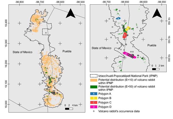
Figure 2 The potential distribution model for R. diazi in the Iztaccíhuatl-Popocatépetl National Park and potential distribution model with the area reduced to those with greater suitability. All the models obtained with the threshold E = 10 or E = 50 were added together, and the pixels where at least 50 % of the models predict presence were selected. On the right side, four polygons (A, B, C, and D) are shown based on the potential distribution model E = 50 and Google Roads map. 

Discussion

Ecological niche modelling and its use as a hypothesis of potential or actual geographical distribution are helpful in prioritizing conservation areas (Sánchez-Cordero et al. 2004). The IPNP is a decreed conservation area; however, administration and management’s decision-making should coincide under a theoretical-practical framework.

The information derived from satellite products is a powerful tool for generating models with better performance on detailed scales (e. g.,Rödder et al. 2016; Vila-Viçosa et al. 2020). In this study, we included the NDVI as an abiotic predictor, although it can also be interpreted as a biotic predictor (He et al. 2015). Different plant species have different leaf anatomy that results in variations in the reflectance captured by remote sensing (He et al. 2009). Although it is possible to find areas with diverse vegetation where the NDVI calculated could be similar, the comparison between studies situated in other geographical regions should be taken cautiously. Identifying georeferenced vegetation and its subsequent relationship with the NDVI values allows the replication of our research. For the future, the addition of NDVI values to flora catalogs, discriminating seasonally, altitudinally, and latitudinally, will facilitate sampling and knowledge of the vegetation of an area and its subsequent relationship with the geographical distribution of animals.

This study included different sets of variables from various data sources to obtain a broader spectrum of information. Because statistical methods controlled the evaluations, and we cannot be ensured that the results of the selected final models guarantee accurate geographic distribution, we decided to combine all the models and select only those pixels where at least half of them coincided with increasing the certainty of the results. Distribution models should be generated with high precision and strictly interpreted not to incur unhelpful or unproductive conservation practices that may put the target species at risk and other taxa. However, a potential distribution model from a suitability model is strongly influenced by the different existing configurations and settings. Thus, it is advisable to use methods that allow standardizing the calibration process of a model.

The distribution of R. diazi showed that the volcano rabbit’s occupation could reach most of the IPNP surface (Martínez-Meyer 2005; Farías et al. 2015). However, this is uncertain, and the IPNP administration does not have the information required to determine the appropriate area for implementing a conservation strategy. For this reason, the search for a more realistic distribution area is necessary to provide that basic knowledge. At a 30-meter m scale, the potential distribution model significantly reduced volcano rabbit occupancy within the IPNP polygon to up to 33 % park’s total area. This difference may be caused by the use of a different scale, but also by the use of different variables or the parameterization of the model, so comparisons should be made with caution.

On the other hand, the environmental predictors used corresponded only to the dry season in México. Therefore, the resulting models can be considered informative for the dry season. However, since R. diazi has a very small home range (Cervantes and Martínez-Vázquez 1996), the distribution of this rabbit will likely be very similar in the rainy season.

Several studies have been published about the volcano rabbit over the past few decades. Velázquez and Bocco (1994) considered agriculture one of the factors that most threatened this species on the Tláloc and Pelado volcanoes. They established areas with different degrees of suitability based on this risk factor. Rizo-Aguilar et al. (2015) showed that vegetation structure and altitudinal range are directly related to the abundance of R. diazi. Moreover, the percentage of meadow cover, short grass, and the scrub cover have a positive relationship with the abundance of the volcano rabbit.

In contrast, the closed forest, tall grass, cattle pasture, hunting, bare terrain, and slope have a negative relationship with its abundance (Hunter and Cresswell 2015). We demonstrated that the suitability and potential distribution are not uniform in the IPNP through modelling techniques and the cross-linking of information with data derived from satellite products. The alpine meadow dominated by Muhlenbergia sp. is the most suitable area for R. diazi in the IPNP, followed by the alpine meadow composed of Muhlenbergia sp. and Calamagrostis tolucensis, both belonging to the Poaceae family. The relationships between the volcano rabbit and plant communities were studied by Velázquez and Heil (1996) in the Pelado and Tláloc volcanoes, where the associations of Festuca tolucensis and Trisetum spicatum-Festuca tolucensis had the greatest abundance of R. diazi. While the floristic study of our work was not the main objective, the inclusion of the plants allowed us to corroborate the importance of alpine meadow without trees in the distribution of R. diazi. Conservation strategies should focus on preserving the alpine meadows in the prioritized polygons, avoiding tourist and unskilled personnel’s access to those specific areas. Human activities in high-mountains ecosystems adversely affect animals (Pęksa and Ciach 2015). The speed of road traffic and the emission of noise in the surrounding areas should be controlled (Garriga et al. 2012), along with other practices to mitigate human impact, such as avoiding the discharge of inorganic and organic waste. In the coming years, scientific studies within the IPNP should be carried out jointly with the park administration and human communities to provide updated tools for decision makers.

Our conservation polygons for R. diazi are based on the most suitable areas and existing access roads in the IPNP because of the significant influx of tourists. Polygons were selected using a remote sensor from three specific dates, so we expected that the vegetation, humidity, and the land surface temperature would change at other times. Besides, our polygons have an average altitude upon 3,800 masl, so they could be helpful in a climate change scenario according to the ascent of the lowest altitudinal limit of the volcano rabbit’s distribution (Anderson et al. 2009). Furthermore, the relative abundance of this rabbit is significantly higher in altitudes above 3,600 masl with abundant bunchgrass cover (Osuna et al. 2021). According to the significant evolutionary units proposed by Osuna et al. (2020), these polygons are located in the area of the Nevada south unit and can also be useful as a natural refugee for genetic management.

Global warming in the medium-long term could lead to changes in the distribution of the volcano rabbit since in the mountains there is an altitudinal temperature gradient that will likely lead species to move uphill (Gottfried et al. 2012). This phenomenon may eventually result in an inability to reach optimal conditions, and the species may become extinct (Colwell et al. 2008). Therefore, we consider that the next step for conserving the teporingo could be selecting the most suitable areas within the IPNP under alternative climate change scenarios.

In addition to the proposed polygons, the most suitable areas identified by niche models should be used as a theoretical and practical basis to propose and execute any conservation strategy in situ. In particular, the vegetation within the reduced distribution of volcano rabbit should be conserved. The meadow with Muhlenbergia sp. is a priority area, and reforestation with pine in them is not advisable.

The boundaries of the IPNP were well designed to protect R. diazi. Although this park has recovered some of its forest covers and has a low amount of transformed area (Aguilar-Tomasini et al. 2020), the conservation of an area does not end with its declaration as a Natural Protected Area. Continuous updating is needed to provide precise conservation tools within protected areas. The abiotic and biotic conditions of the park polygon will vary. The methodological tools in the future will provide various techniques that will enable the rise of information about one of the most threatened and emblematic lagomorphs of México: the volcano rabbit.

Literature cited

Aguilar-Tomasini, M. A., T. Escalante, and M. Farfán. 2020. Effectiveness of natural protected areas for preventing land use and land cover changes of the Transmexican Volcanic Belt, Mexico. Regional Environmental Change 20:1-9. [ Links ]

Akaike, H. 1974. A new look at the statistical model identification. IEEE Transactions on Automatic Control 19:716-723. [ Links ]

Anderson, B. J., H. R. Akçakaya, M. B. Araújo, D. A. Fordham, E. Martínez-Meyer, W. Thuiller, and B. W. Brook. 2009. Dynamics of range margins for metapopulations under climate change. Proceedings of the Royal Society B: Biological Sciences 276:1415-1420. [ Links ]

Ariza, A. 2013. Descripción y Corrección de Productos Landsat 8 LDCM (Landsat Data Continuity Mission). Bogotá Instituto Geográfico Agustín Codazzi. [ Links ]

Austin, M. 2007. Species distribution models and ecological theory: A critical assessment and some possible new approaches. Ecological Modelling 200:1-19. [ Links ]

Avdan, U., and G. Jovanovska. 2016. Algorithm for automated mapping of land surface temperature using LANDSAT 8 satellite data. Journal of Sensors 2016. [ Links ]

Barrera, A. 1966. Redefinición de Cediopsylla Jordán y Hoplopyllus nuevas especies, comentarios sobre el concepto de relicto y un caso de evolución convergente. Revista de la Sociedad Mexicana de Historia Natural 27:67-83. [ Links ]

Barsi, J. A., J. R. Schott, S. J. Hook, N. G. Raqueno, B. L. Markham, and R. G. Radocinski. 2014. Landsat-8 thermal infrared sensor (TIRS) vicarious radiometric calibration. Remote Sensing 6:11607-11626. [ Links ]

Burnham, K. P., and D. R. Anderson. 2002. Model selection and multimodel inference: a practical information-theoretic approach. 2nd ed. Springer-Verlag. Berlin, Germany. [ Links ]

Carlson, T. N., and D. A. Ripley. 1997. On the relation between NDVI, fractional vegetation cover, and leaf area index. Remote Sensing of Environment 62:241-252. [ Links ]

Cervantes, F. A. 1982. Observaciones sobre la reproducción del zacatuche o teporingo Romerolagus diazi. Mammalia: Lagomorpha. Doñana Acta Vertebrata 9:416-420. [ Links ]

Cervantes, F. A., and J. Martínez-Vázquez. 1996. Historia natural del conejo zacatuche o teporingo (Romerolagus diazi). Pp. 29-40, in Ecología y Conservación del conejo zacatuche y su hábitat (Velázquez, A., F. Romero, and J. López-Paniagua, eds.). Universidad Autónoma de México-Fondo de Cultura Económica. Mexico City, Mexico. [ Links ]

Chamberlain, S., V. Barve, D. Mcglinn, D. Oldoni, P. Desmet, L. Geffert, and K. Ram. 2020. rgbif: Interface to the Global Biodiversity Information Facility API. [ Links ]

Cobos, M. E., A. T. Peterson, N. Barve, and L. Osorio-Olvera. 2019. Kuenm: An R package for detailed development of ecological niche models using Maxent. PeerJ 2019:1-15. [ Links ]

Colwell, R. K., G. Brehm, C. L. Cardelús, A. C. Gilman, J. T. Longino, C. L. Cardelus, A. C. Gilman, and J. T. Longino. 2008. Global Warming, Elevational Range Shifts, and Lowland Biotic Attrition in the Wet Tropics. Science 322:258-261. [ Links ]

Comisión Nacional de Áreas Naturales Protegidas (CONANP). 2013. Programa de manejo Parque Nacional Iztaccíhuatl-Popocatépetl. Mexico City, Mexico. [ Links ]

Dash, P., F. M. Göttsche, F. S. Olesen, and H. Fischer. 2005. Separating surface emissivity and temperature using two-channel spectral indices and emissivity composites and comparison with a vegetation fraction method. Remote Sensing of Environment 96:1-17. [ Links ]

Escalante, T. 2014. Modelos de distribución de especies de mamíferos y suculentas de la Faja Volcánica Transmexicana. Database SNIB-CONABIO_Mamíferos, project JM055. Universidad Nacional Autónoma de México. Facultad de Ciencias. Mexico City, Mexico. [ Links ]

Farías, V., Y. García-Feria, O. Téllez-Valdés, and V. Bernal-Legaria. 2015. ‘Romerolagus diazi (zacatuche). Distribución potencial.’, escala: 1:1000000, in Distribución potencial de las especies de Leporidae en México y las implicaciones para su conservación., project: JM034, Facultad de Estudios Superiores Iztacala, Universidad Nacional Autónoma de México. Mexico City, Mexico. [ Links ]

Galindo-Leal, C., and A. Velázquez. 1996. Recomendaciones para la conservación del zacatuche. Pp. 147-157, in Ecología y Conservación del conejo zacatuche y su hábitat (Velázquez, A. , F. Romero, and J. López-Paniagua, eds.). Universidad Nacional Autónoma de México-Fondo de Cultura Económica. Mexico City, Mexico. [ Links ]

Garriga, N., X. Santos, A. Montori, A. Richter-Boix, M. Franch, and G. Llorente. 2012. Are protected areas truly protected? The impact of road traffic on vertebrate fauna. Biodiversity and Conservation 21:2761-2774. [ Links ]

Google Incorporated. 2019. Google Roads. [ Links ]

Gottfried, M., H. Pauli, A. Futschik, M. Akhalkatsi, P. Barančok, J. L. Benito Alonso, G. Coldea, J. Dick, B. Erschbamer, M. R. Fernández-Calzado, G. Kazakis, J. Krajči, P. Larsson, M. Mallaun, O. Michelsen, D. Moiseev, P. Moiseev, U. Molau, A. Merzouki, L. Nagy, G. Nakhutsrishvili, B. Pedersen, G. Pelino, M. Puscas, G. Rossi, A. Stanisci, J. P. Theurillat, M. Tomaselli, L. Villar, P. Vittoz, I. Vogiatzakis, and G. Grabherr. 2012. Continent-wide response of mountain vegetation to climate change. Natural Climate Change 2:111-115. [ Links ]

He, K. S., B. A. Bradley, A. F. Cord, D. Rocchini, M. N. Tuanmu, S. Schmidtlein, W. Turner, M. Wegmann, and N. Pettorelli. 2015. Will remote sensing shape the next generation of species distribution models? Remote Sensing in Ecology and Conservation 1:4-18. [ Links ]

He, K. S. , J. Zhang, and Q. Zhang. 2009. Linking variability in species composition and MODIS NDVI based on beta diversity measurements. Acta Oecologica 35:14-21. [ Links ]

Hijmans, R. J., S. Phillips, J. Leathwick, V. J. Elith, and M. R. J. Hijmans. 2017. Package ‘dismo.’ Circles 9:1-68. [ Links ]

Hoffman, A., F. Cervantes, and J. Morales-Malacara. 1994. Ectoparásitos del conejo zacatuche (Romerolagus diazi). Anales del Instituto de Biología 65:209-215. [ Links ]

Hunter, M., and W. Cresswell. 2015. Factors affecting the distribution and abundance of the Endangered volcano rabbit Romerolagus diazi on the Iztaccihuatl volcano. Oryx 49:366-375. [ Links ]

Instituto Nacional de Estadística y Geografía (INEGI). 2010. Censo de Población y Vivienda 2010. Principales resultados por localidad (ITER). Mexico. [ Links ]

Instituto Nacional de Estadística y Geografía (INEGI). 2013. Continuo de Elevaciones Mexicano (CEM). http://www.beta.inegi.org.mx/app/geo2/elevacionesmex/Links ]

Lawler, J. J., D. White, J. C. Sifneos, and L. L. Master. 2003. Rare species and the use of indicator groups for conservation planning. Conservation Biology 17:875-882. [ Links ]

Lobo, J. M., A. Jiménez-Valverde, and R. Real. 2008. AUC: A misleading measure of the performance of predictive distribution models. Global Ecology and Biogeography 17:145-151. [ Links ]

Martínez-Meyer, E. 2005. Climate change and biodiversity: some considerations in forecasting shifts in species’ potential distributions. Biodiversity Informatics 2:42-55. [ Links ]

Mateo, R. G., Á. M. Felicísimo, and J. Muñoz. 2011. Modelos de distribución de especies: Una revisión sintética. Revista Chilena de Historia Natural 84:217-240. [ Links ]

Merow, C., M. J. Smith, and J. A. Silander. 2013. A practical guide to MaxEnt for modeling species’ distributions: What it does, and why inputs and settings matter. Ecography 36:1058-1069. [ Links ]

Montgomery, D., and E. Peck. 1992. Introduction to linear regression analysis. 2nd ed. Wiley. New York, U. S. A. [ Links ]

Muscarella, R., P. J. Galante, M. Soley-Guardia, R. A. Boria, J. M. Kass, M. Uriarte, and R. P. Anderson. 2014. ENMeval: An R package for conducting spatially independent evaluations and estimating optimal model complexity for Maxent ecological niche models. Methods in Ecology and Evolution 5:1198-1205. [ Links ]

Osorio-Olvera, L., A. Lira-Noriega, J. Soberón, A. T. Peterson, M. Falconi, R. G. Contreras-Díaz, E. Martínez-Meyer, V. Barve, and N. Barve. 2020. ntbox: An r package with graphical user interface for modelling and evaluating multidimensional ecological niches. Methods in Ecology and Evolution 2020 11:1199-1206. [ Links ]

Osuna, F., D. González, A. E. de los Monteros, and J. A. Guerrero. 2020. Phylogeography of the Volcano Rabbit (Romerolagus diazi): the Evolutionary History of a Mountain Specialist Molded by the Climatic-Volcanism Interaction in the Central Mexican Highlands. Journal of Mammalian Evolution 27:745-757. [ Links ]

Osuna, F. , R. Guevara, E. Martínez-Meyer, R. Alcalá, and A. E. de los Monteros. 2021. Factors affecting presence and relative abundance of the Endangered volcano rabbit Romerolagus diazi, a habitat specialist. Oryx 1-10. [ Links ]

Peterson, A. T., M. Papeş, and J. Soberón. 2008. Rethinking receiver operating characteristic analysis applications in ecological niche modeling. Ecological Modelling 213:63-72. [ Links ]

Pęksa, Ł., and M. Ciach. 2015. Negative effects of mass tourism on high mountain fauna: the case of the Tatra chamois Rupicapra rupicapra tatrica. Oryx 49:500-505. [ Links ]

Phillips, S. J., R. P. Anderson, and R. Schapire. 2006. Maximum entropy modeling of species geographic distributions. Ecological Modelling 190:231-259. [ Links ]

Phillips, S. J. , R. P. Anderson, M. Dudík, R. E. Schapire, and M. E. Blair. 2017. Opening the black box: an open-source release of Maxent. Ecography 40:887-893. [ Links ]

Prieto-Torres, D. A., and G. Pinilla-Buitrago . 2017. Estimating the potential distribution and conservation priorities of Chironectes minimus (Zimmermann, 1780) (Didelphimorphia: Didelphidae). Therya 8:131-144. [ Links ]

QGIS Development Team. 2019. QGIS Geographic Information System. Open Source Geospatial Foundation Project. [ Links ]

Radosavljevic, A., and R. P. Anderson. 2014. Making better Maxent models of species distributions: Complexity, overfitting and evaluation. Journal of Biogeography 41:629-643. [ Links ]

Rizo-Aguilar, A., J. A. Guerrero, M. G. Hidalgo-Mihart, and A. González-Romero. 2015. Relationship between the abundance of the Endangered volcano rabbit Romerolagus diazi and vegetation structure in the Sierra Chichinautzin mountain range. Oryx 49:360-365. [ Links ]

Rizo-Aguilar, A. , J. A. Guerrero, A. M. P. Montoya-Lara , and C. Valdespino. 2014. Physiological stress in volcano rabbit Romerolagus diazi populations inhabiting contrasting zones at the Corredor Biologico Chichinautzin, Mexico. Mammalian Biology 79:357-361. [ Links ]

Rödder, D., S. Nekum, A. F. Cord, and J. O. Engler. 2016. Coupling Satellite Data with Species Distribution and Connectivity Models as a Tool for Environmental Management and Planning in Matrix-Sensitive Species. Environmental Management 58:130-143. [ Links ]

Rouse, J., R. Haas, J. Schell, and D. Deerin. 1973. Monitoring vegetation systems in the Great Plains with ERTS. N. SP-351. Pp. 309-317, in Third ERTS Symposyum. NASA. Washington, U.S.A. [ Links ]

RStudio Team. 2018. RStudio: Integrated Development Environment for R. RStudio, Inc. Boston, U. S. A. [ Links ]

Sánchez-Cordero, V., M. Munguia, and A. T. Peterson. 2004. GIS-based predictive biogeography in the context of conservation. Pp. 311-323, in Frontiers of biogeography: new directions in the geography of nature (Lomolino, M. V., and L. R. Heaney, eds.). Sinauer Associates, Inc. Massachusetts, U. S. A. [ Links ]

Secretaria de Medio Ambiente y Recursos Naturales (SEMARNAT). 2013. Diario Oficial. Acuerdo por el que se da a conocer el resumen del Programa de Manejo del Parque Nacional Iztaccíhuatl−Popocatépetl. Mexico. [ Links ]

Soberón, J., L. Osorio-Olvera, and A. T. Peterson. 2017. Diferencias conceptuales entre modelación de nichos y modelación de áreas de distribución. Revista Mexicana de Biodiversidad 88:437-441. [ Links ]

Soberón, J. , and A. T. Peterson . 2005. Interpretation of models of fundamental ecological niches and species’ distributional areas. Biodiversity Informatics 2:1-10. [ Links ]

Sobrino, J. A., and N. Raissouni. 2000. Toward remote sensing methods for land cover dynamic monitoring: Application to Morocco. International Journal of Remote Sensing 21:353-366. [ Links ]

Sobrino, J. A. , J. C. Jiménez-Muñoz, and L. Paolini. 2004. Land surface temperature retrieval from LANDSAT TM 5. Remote Sensing of Environment 90:434-440. [ Links ]

Sobrino, J. A. , J. C. Jiménez-Muñoz, G. Sòria, M. Romaguera, L. Guanter, J. Moreno, A. Plaza, and P. Martínez. 2008. Land surface emissivity retrieval from different VNIR and TIR sensors. IEEE Transactions on Geoscience and Remote Sensing 46:316-327. [ Links ]

Stathopoulou, M., and C. Cartalis. 2007. Daytime urban heat islands from Landsat ETM+ and Corine land cover data: An application to major cities in Greece. Solar Energy 81:358-368. [ Links ]

TEAM Network. 2017. Tropical Ecology Assessment and Monitoring Network. [ Links ]

United States Geological Survey (USGS). 2013. Landsat Missions. https://www.usgs.gov/land-resources/nli/landsat. [ Links ]

United States Geological Survey (USGS). 2019. Landsat 8. https://earthexplorer.usgs.gov/. [ Links ]

Velazquez, A., and G. Bocco. 1994. Modelling conservation alternatives with ILWIS: a case study of the volcano rabbit. ITC Journal 3:197-204. [ Links ]

Velázquez, A. , and J. A. Guerrero . 2019. Romerolagus diazi. The IUCN Red List of Threatened Species 2019: e.T19742A45180356. [ Links ]

Velázquez, A. , F. Romero, and L. León . 1996. Fragmentación del hábitat del conejo zacatuche. Pp. 73-86, in Ecología y Conservación del conejo zacatuche y su hábitat (Velázquez, A. , F. Romero, and J. López-Paniagua, eds.). Universidad Nacional Autónoma de México-Fondo de Cultura Económica. Mexico City, Mexico. [ Links ]

Velazquez, A. , and G. W. Heil. 1996. Habitat Suitability Study for the Conservation of the Volcano Rabbit (Romerolagus diazi). Journal of Applied Ecology 33:543-554. [ Links ]

Vila-Viçosa, C., S. Arenas-Castro, B. Marcos, J. Honrado, C. García, F. M. Vázquez, R. Almedia, and J. Gonçalves. 2020. Combining Satellite Remote Sensing and Climate Data in Species Distribution Models to Improve the Conservation of Iberian White Oaks (Quercus L.). International Journal of Geo-Information 9:735. [ Links ]

Waltari, E., and R. P. Guralnick. 2008. Ecological niche modelling of montane mammals in the Great Basin, North America: examining past and present connectivity of species across basins and ranges. Journal of Biogeography 36:148-161. [ Links ]

Wang, F., Z. Qin, C. Song, L. Tu, A. Karnieli, and S. Zhao. 2015. An improved mono-window algorithm for land surface temperature retrieval from landsat 8 thermal infrared sensor data. Remote Sensing 7:4268-4289. [ Links ]

Warren, D. L., and S. N. Seifert. 2011. Ecological niche modeling in Maxent: The importance of model complexity and the performance of model selection criteria. Ecological Applications 21:335-342. [ Links ]

0Associated editor: Lázaro Guevara

Appendix 1

Abraczinskas, L. 2016. MSU Mammalogy, Ornithology and Vertebrate Paleontology Collections. Version 8.1. Michigan State University Museum.

Arroyo-Cabrales, J. 2018a. Mexican mammals in safekeeping of The Natural History Museum (London), England. Version 1.5. Comisión Nacional para el conocimiento y uso de la Biodiversidad.

Arroyo-Cabrales, J. 2018b. La mastofauna del cuaternario tardío de México. Version 1.5. Comisión Nacional para el conocimiento y uso de la Biodiversidad.

Bucci, M. 2016. UAZ Mammals. Version 5.1. University of Arizona Museum of Natural History.

Cano-Reveles, J. 2018. Restauración, protección y manejo de ecosistemas del Parque Nacional Pico de Orizaba y su área de influencia, in collaboration with SEMARNAT, CONANP, CONAFOR and PROFEPA. Version 1.5. Comisión Nacional para el conocimiento y uso de la Biodiversidad.

Ceballos-González, G. 2018. Database update from Atlas Mastozoológico de México. Comisión Nacional para el conocimiento y uso de la Biodiversidad.

Cervantes, F. 2018a. Database update of State of Morelos from Colección Nacional de Mamíferos del Instituto de Biología, UNAM. Version 1.5. Comisión Nacional para el conocimiento y uso de la Biodiversidad.

Cervantes, F. 2018b. Bar codes of specimens from Colección Nacional de Mamíferos del Instituto de Biología, UNAM. Version 1.5. Comisión Nacional para el conocimiento y uso de la Biodiversidad.

Conroy, C. 2019. MVZ Mammal Collection (Arctos). Version 35.25. Museum of Vertebrate Zoology.

Escobar-Ocampo, M. 2018. Sistematización de las colecciones científicas del Instituto de Historia Natural y Ecología, (IHNE) Chiapas Comisión Nacional para el conocimiento y uso de la Biodiversidad.

Garner, H. 2016. TTU Mammals Collection. Version 9.1. Museum of Texas Tech University (TTU).

Grant, S. and A. Ferguson. 2019. Field Museum of Natural History (Zoology) Mammal Collection. Version 9.6. Field Museum.

iNaturalist.org. 2019. iNaturalist Research-grade Observations.

Kurta, A. 2018. T. L. Hankinson Vertebrate Museum (EMU) Mammal Collection. T. L. Hankinson Vertebrate Museum, Eastern Michigan.

León-Paniagua, L. 2018. Database update from Colección de mamíferos del Museo de Zoología ‘Alfonso L. Herrera’. Version 1.5. Comisión Nacional para el conocimiento y uso de la Biodiversidad.

López-Vidal, J. 2018a. Computarización de las colecciones de vertebrados terrestres de la Escuela Nacional de Ciencias Biológicas, IPN - Fases 2 y 3. Comisión Nacional para el conocimiento y uso de la Biodiversidad.

López-Vidal, J. 2018b. Computarización de las colecciones de vertebrados terrestres de la Escuela Nacional de Ciencias Biológicas, IPN Fase 1: Estado de México, Hidalgo, San Luis Potosí y Tlaxcala. Comisión nacional para el conocimiento y uso de la biodiversidad.

López-Wilchis, R. 2018. Base de datos de mamíferos de México depositados en colecciones de Estados Unidos y Canadá. Version 1.5. Comisión Nacional para el conocimiento y uso de la Biodiversidad.

Magaña-Cota, G. 2018. Scientific collection from Museo de Historia Natural Alfredo Dugés. Comisión Nacional para el conocimiento y uso de la Biodiversidad.

McCormack, J. 2019. MLZ Mammal Collection (Arctos). Version 33.24. Moore Laboratory of Zoology.

Morris, P. 2019. Museum of Comparative Zoology, Harvard University. Version 162.146. Harvard University Museum. Museum of Comparative Zoology, Harvard University.

Natural History Museum. 2019. Natural History Museum (London) Collection Specimens.

Prestridge, H. 2018. Biodiversity Research and Teaching Collections - TCWC Vertebrates. Version 9.2. Texas A&M University Biodiversity Research and Teaching Collections.

Royal Belgian Institute of Natural Sciences. 2017. RBINS DaRWIN.

Orrell, T. and T. Hollowell. 2018. NMNH Extant Specimen Records. Version 1.19. National Museum of Natural History, Smithsonian Institution.

Ramírez-Pulido, J. 2018. Biodiversidad mastozoológica del Eje Volcánico Transversal. Version 1.5. Comisión Nacional para el conocimiento y uso de la Biodiversidad.

Sánchez-Cordero, V. 2018. Fortalecimiento de la Colección de fotocolectas biológicas (CFB): una propuesta del uso de la imagen digital al servicio del conocimiento de la biodiversidad. Versión 1.5. Comisión Nacional para el conocimiento y uso de la Biodiversidad.

Schmidt, C. 2016. FHSM Mammals Collection. Fort Hays Sternberg Museum of Natural History.

Slade, N. 2019. KUBI Mammalogy Collection. Version 26.20. University of Kansas Biodiversity Institute.

Trombone, T. 2016. AMNH Mammal Collections. American Museum of Natural History.

University of Michigan Museum of Zoology. 2019. University of Michigan Museum of Zoology, Division of Mammals. Version 8.5.

Velázquez-Montes, J. 2018. Análisis de la heterogeneidad ambiental y conectividad de las áreas naturales del sur del Valle de México. Comisión nacional para el conocimiento yuso de la biodiversidad.

Appendix 2

#Correlations (Marco F. Ortiz and David Prieto-Torres)

library(sp)

library(raster)

library(rgeos)

library(maptools)

library(rgdal)

library(usdm)

library(foreign)

library(rJava)

library(spocc)

library(corrplot)

library(usdm)

rm(list=ls())

setwd(“C:/Work_directory_with_climate_layers”)

pca_path <- list.files(“.”,pattern = “*.asc$”,full.names = T)

climatelayers<- stack(pca_path)

setwd(“C:/Work_directory_with_presence_data”)

data <- read.csv(“species.csv”)

plot(climatelayers[,1])

species<-data$species

lat<-data$y

lon<-data$x

Specie_estudied<-data.frame(species,lon,lat)

presences_climate <- data.frame(extract(climatelayers,Specie_estudied[,2:3]))

presences_climate2<-data.frame(Specie_estudied, presences_climate)

presences_climate3 <- na.omit(presences_climate2)

setwd(“C:/Work_directory_presence_with_climate”)

write.csv(presences_climate3[,1:3], file = “name.csv”)

### Collinearity matrix and VIF estimation##

cormatriz <- cor(presences_climate3[,4:22]) ##bio1-bio19##

setwd(“C:/work_directory”)

windows()

corrplot(cormatriz, outline = T, tl.col = “black”, mar = c(2,0,1,1.5), title = “title”)

###VIF>10 [Montgomery and Peck (1992)]

vif(presences_climate2[,4:22])

no_corr <- vifstep(presences_climate2[,4:22], th=10)

no_corr

Appendix 3

Geographic decimal coordinates of the proposed polygons for conservation of Romerolagus diazi within Iztaccihuatl-Popocatepetl National Park.

Vortex Longitude Latitude
Polygon A    
1 -98.670676 19.15410191
2 -98.673186 19.15465969
3 -98.6740227 19.15521747
4 -98.6743016 19.15549636
5 -98.6743016 19.15577525
6 -98.6740227 19.15689082
7 -98.6737438 19.15716971
8 -98.6729071 19.15772749
9 -98.6723494 19.15800638
10 -98.6664927 19.16079528
11 -98.6662138 19.16079528
12 -98.6617515 19.15828527
13 -98.6611938 19.1574486
14 -98.6611938 19.1571697
15 -98.6637038 19.1546596
16 -98.6642615 19.1543808
17 -98.6650982 19.1541019
Polygon B    
1 -98.647807 19.12342401
2 -98.6492015 19.12426068
3 -98.6492015 19.12565513
4 -98.6425081 19.13513739
5 -98.6419503 19.13569517
6 -98.6405559 19.13569517
7 -98.6346992 19.13067515
8 -98.6344203 19.13039626
9 -98.6344203 19.12983848
10 -98.6355359 19.12816514
11 -98.6358147 19.12788625
12 -98.6466915 19.12342401
Polygon C    
1 -98.6514326 19.10278614
2 -98.6547793 19.1039017
3 -98.6553371 19.10418059
4 -98.6558948 19.10473837
5 -98.6561737 19.10529615
6 -98.6561737 19.10585393
7 -98.6558948 19.10780616
8 -98.6533848 19.11589397
9 -98.652827 19.11700953
10 -98.6508748 19.11979843
11 -98.6494804 19.11979843
12 -98.6475281 19.11896176
13 -98.6447392 19.11617286
Vortex Longitude Latitude
14 -98.6444603 19.11589397
15 -98.6444603 19.11533619
16 -98.6455759 19.10724838
17 -98.6461337 19.1066906
18 -98.647807 19.10501726
19 -98.6511537 19.10278614
Polygon D    
1 -98.6215913 19.04840257
2 -98.6268903 19.04896035
3 -98.6413925 19.05481705
4 -98.6505959 19.05955818
5 -98.6553371 19.06206819
6 98.655616 19.06234708
7 -98.6558948 19.06318375
8 -98.6558948 19.06374153
9 -98.6505959 19.0673671
10 -98.650317 19.0673671
11 -98.6254958 19.05649039
12 -98.6188024 19.05258592
13 -98.6188024 19.05147036
14 -98.6213125 19.04840257

Received: November 12, 2020; Revised: February 21, 2021; Accepted: June 23, 2021

*Corresponding author: luisjose@ciencias.unam.mx

Creative Commons License This is an open-access article distributed under the terms of the Creative Commons Attribution License