




Services on Demand
Journal
Article
 text in
 English (pdf)
 Article in xml format
 Article references

 Automatic translation
 Send this article by e-mail
Indicators
-
 Cited by SciELO
-
 Access statistics
Related links
-
 Similars in
SciELO
Share

 Permalink

Tecnología y ciencias del agua
On-line version ISSN 2007-2422
Tecnol. cienc. agua vol.12 n.3 Jiutepec May./Jun. 2021 Epub June 26, 2025
https://doi.org/10.24850/j-tyca-2021-03-05
Articles
Fitting of non-stationary distribution GEV11 through L moments
1Profesor jubilado de la Universidad Autónoma de San Luis Potosí, San Luis Potosí, México, campos_aranda@hotmail.com
Hydrological dimensioning or revision of the hydraulic works and the elaboration of flood risk maps is based on the so-called Design Floods, which are maximum flows of the river associated with low probabilities of exceedance. The most reliable way of estimating such predictions is through Flood Frequency Analysis (FFA). Its fundamental assumption is that the stochastic process under study is stationary, i.e., it does not change with time. Construction of reservoirs, urbanization and changes in land use in the basin, as well as global or regional climate change, alter the hydrological processes and generate records of annual flows that are non-stationary, showing trends and changes in variability. For the FFA of such registries, the extreme value theory has been extended to apply its classical distribution, the Generalized Extreme Values (GEV), with parameters of location (u) and scale (α) varying with time (t), which is introduced as a covariate. In this work the L-moment method is presented for the fit of the probabilistic model GVE11 whose parameters u and α vary linearly over time. Three numerical applications are described. Conclusions highlight the simplicity of the exposed method and its importance in the estimation of the expected predictions in non-stationary annual maximum data series.
Keywords: Covariate; L-moments; GEV distribution; standard error of fit; trend; linear regression; residuals
El dimensionamiento o la revisión hidrológica de las obras hidráulicas y la elaboración de mapas de riesgo por inundación se realizan con base en las llamadas crecientes de diseño, que son gastos máximos del río asociados con bajas probabilidades de excedencia. La manera más confiable de estimar tales predicciones es a través del Análisis de Frecuencias de Crecientes (AFC), cuya suposición fundamental es que el proceso estocástico bajo estudio es estacionario, es decir, que no cambia con el tiempo. La construcción de embalses pequeños, la urbanización y los cambios de uso del suelo en la cuenca, así como el cambio climático global o regional alteran los procesos hidrológicos y generan registros de crecientes anuales que son no estacionarios, al mostrar tendencias y cambio en su variabilidad. Para el AFC de tales registros se ha extendido la teoría de valores extremos, a fin de aplicar su distribución clásica, la General de Valores Extremos (GVE), con parámetros de ubicación (u) y escala (a) variables con el tiempo (t), que se introduce como covariable. En este trabajo se expone el método de momentos L para el ajuste del modelo probabilístico GVE11, cuyos parámetros u y α varían linealmente con el tiempo. Se describen tres aplicaciones numéricas. Las conclusiones destacan la sencillez del método expuesto y su importancia en la estimación de las predicciones buscadas en series de datos máximos anuales no estacionarios.
Palabras clave: covariable; momentos L; distribución GVE; error estándar de ajuste; tendencia; regresión lineal; residuales
Introduction
Flood risk estimation of a certain area and hydrological dimensioning of water works: reservoirs, bridges, walls and protective embankments and channelings, is carried out based on so-called Design Floods, which are extreme flows of the river associated with low Exceedance Probability. The most reliable estimation of design floods is carried out through Flood Frequency Analysis (FFA) of the available record or series of maximum annual flows. FFA assumes that the random process that generates such floods is stationary and therefore its statistical properties do not change over time (Khaliq, Ouarda, Ondo, Gachon, & Bobée, 2006; El-Adlouni, Ouarda, Zhang, Roy, & Bobée, 2007; El-Adlouni & Ouarda, 2008).
All physical changes that occur in drainage basins, such as the construction of reservoirs, urbanization, channel straightening, deforestation, and land use change alter the hydrological processes, giving rise to series or records of non-stationary annual maximum flows, because they present trends and changes in variability. In addition, the impacts of global climate change can exacerbate hydrological process alterations, favoring the formation of non-stationary extreme hydrological data sets. Since early 1990s, non-stationarity due to urbanization and/or climate change was taken into account, correcting the available records, applying incremental factors to predictions, or making predictions in the rural basin and then adjusting the results for their level of urbanization (Jakob, 2013; Prosdocimi, Kjeldsen, & Miller, 2015).
Currently, the statistical Extreme Value Theory (EVT) has been extended to non-stationary conditions, to fit the classical distribution that follow asymptotically the maximum hydrological data series, i.e. the stationary probabilistic model Generalized Extreme Value (GEV0) with three fitting parameters (u,α,k). This is based on the introduction of the so-called covariates, and one of the most used is time (t) in years, through which the trend observed in data series can be taken into account, adopting the location parameter variable (ut ). When the trend is linear, ut =μ0+μ1·t and then the four fitting parameter GVE1 model is fitted (μ0,μ1,α,k). If the trend is curve, ut =μ0+μ1·t+μ2·t2 and the five fitting parameter GVE2 model is applied (μ0,μ1,μ2,α,k). In the GVE11 model, both the location parameter and the scale parameter (αt =σ0+σ1·t) are linear functions of t time and then, in addition to the trend, the change over time of series variability is considered (Khaliq et al., 2006; El-Adlouni & Ouarda, 2008; Aissaoui-Fqayeh, El-Adlouni, Ouarda, & St. Hilaire, 2009; Jakob, 2013; Gado & Nguyen 2016).
Khaliq et al. (2006), and Meylan, Favre and Musy (2012) have presented a review of various methods used in FFA, in the non-stationary context. Such techniques include the incorporation of trends in distribution parameters or at statistical moments, the quantile regression method, local likelihood processes, and the Bayesian approach. In the probabilistic models of the first approach, the use of covariates aims to integrate changes that have occurred in the past directly into the techniques of FFA, with the aim of extrapolating them to the future. In this context, models that use time as a covariate, case of the one presented here, are simple and useful to reproduce the non-stationary behavior of a flood record, but the acceptance of their predictions is not entirely correct, given that, as indicated by López and Francés (2013), trends may change in the short or long term, due to climate variability or the intensification of human activities.
Due to the above, the possibility of incorporating climate indices as external forcing into the FFA models has been explored over the past two decades, assuming linear or non-linear dependence. This approach has shown that the use of such covariates leads to models that better describe temporal changes occurred in flood records. In fact, a remote connection has been found between the observed changes in flood regimes and the anomalies in the indices (ENSO: El Niño-Southern Oscillation; PDO: Pacific Decadal Oscillation and NAO: North Atlantic Oscillation) describing the temporal evolution of low-frequency atmospheric circulation patterns (Khaliq et al., 2006; López-de-la-Cruz & Francés, 2014).
The objective of this work was to expose the theory of fitting Generalized Extreme Values (GEV) distribution in non-stationary conditions, by generalizing the L-moment method, proposed by Gado and Nguyen (2016) for the GVE11 model. Three series of extreme hydrological data taken from the specialized literature are exposed and processed, and their results discussed, highlighting the simplicity and usefulness of the L-moment method to obtain predictions within the historical and future record, when they are important, due to the series upward trend and/or its increasing variability.
Operational theory
Generalized Extreme Values Distribution
Annual extreme values are rare events occurring in the right extremity or tail of the probability distribution function (PDF), which is the probabilistic model that defines the behavior of the hydrological random variable under study, such as: floods and maximum values of rainfalls, temperatures, winds and sea levels. The extreme values can be predicted based on the PDF, such as the maximum of the random variable that corresponds to a certain average interval of recurrence or period of return (Tr), whose exceedance probability is p = 1/Tr.
Extreme value theory justifies and states that extreme data follows in an asymptotic manner any of the three types of distributions called: Gumbel, Fréchet or Weibull (Clarke, 1973; Stedinger, Vogel, & Foufoula-Georgiou, 1993; Coles, 2001; Khaliq et al., 2006). These three probabilistic models can be represented in one, called Generalized Extreme Value distribution (GEV), whose application has been widely recommended for modeling annual maximum flows (q) and other extreme data (Hosking & Wallis, 1997; Papalexiou & Koutsoyiannis, 2013; Gado & Nguyen, 2016; Stedinger, 2017). The PDF of the GEV with a non-exceedance probability [F(q)] is:
In the above expression, u, α, and k are the location, scale, and shape parameters of the GEV distribution. When k = 0 the Gumbel distribution is obtained, which is a straight line on the Gumbel-Powell probability paper (Chow, 1964), so the interval of the variable is: -∞ < q < ∞. When k > 0 the distribution is Weibull, which is a curve with downward concavity and upper limit, so: -∞ < q ≤ u + α / k. Finally, if k < 0 the distribution is Fréchet, which is also a curve, but with an upward concavity and lower border, so: u + α / k ≤ q <∞. The expected predictions (QTr ) are obtained with the inverse solution of Equation (1):
Data sample L-moments
L-moment method is perhaps the simplest one, and it has become one of the reliable procedures for estimating the PDF fitting parameters used in hydrology. This is because L-moments, which are linear combinations (Hosking & Wallis, 1997) of weighted probability moments (βr ), are not significantly affected by sample outliers. The first three L-moments of a sample (l1, l2, l3) and the asymmetry L-ratio (t3) are estimated by the unbiased estimator (br ) of the βr , as follows:
The unbiased estimator of the βr is (Hosking & Wallis, 1997):
where r = 0, 1, 2,…. and qj are the data of the available sample or series of size n, ordered from minor to major
Stationary GEV distribution fitting parameters
With the L-moment method for the GVE0 model, the following equations are obtained for its three fitting parameters (Stedinger et al., 1993; Hosking & Wallis, 1997; Rao & Hamed, 2000; Stedinger, 2017):
being:
The Stirling formula (Davis, 1972) was used to estimate the value of Gamma Γ(ω) function:
Non-stationary analysis approach
It has two inherent assumptions, the first accepts that non-stationarity of the hydrological series of extreme annual values is caused by gradual changes in land use or by global or regional climate change; generating a slight alteration of its statistical parameters. The second assumption accepts that the PDF is time-independent, so the GEV distribution, with variable fitting parameters over time, is acceptable for modeling extreme non-stationary data.
Due to non-stationarity, there is great statistical variability associated with the sample or series of available extreme annual data and it is therefore appropriate to adopt that mean (μ) and standard deviation (σ) are functions of time. The simplest way, is carried out by means of the probabilistic model GEV11 with linear variations, so: μt =μ0+μ1·t and ln(σt )=σ0+σ1·t. In the above expressions, t is the time-in-years covariate that encompasses the n-size data series. The use of natural logarithms of σ ensures positive values of the scale parameter (α) in the GEV distribution (Gado & Nguyen, 2016). The general expressions of the mean and standard deviation of the GEV0 model, the second one obtained through the second central moment, are (Rao & Hamed, 2000):
GEV11 distribution fitting
Since the mean and the natural logarithm of the standard deviation are linear functions of time, the expression: μt =μ0+μ1·t is first entered in Equation (13) to clear the variable location parameter expression over time (ut ), in which the scale parameter (αt ) is also variable, and where FK1 is the first function factor of the form parameter (k), such an equation is (Gado & Nguyen, 2016):
where:
From Equation (14), you get the variable scale parameter expression over time:
So:
being:
Substituting Equation (18) in the Equation (15), the variable scale parameter expression over time is obtained:
The magnitudes μ0 and μ1 of the straight line representing the linear trend of the sample or data series qt are obtained based on the equations of the linear regression straight line, as follows. The dependent variable (y) is considered to be the maximum annual hydrological data qt and the times or years t are the abscissa (x), in this case equal to the i-th value of i. The slope (μ1) of the regression straight line adjusted by least squares of the residuals and the y-intercept (μ0) are obtained with the following equations (Campos-Aranda, 2003):
In the equations above,
being:
To estimate the linear trend in the standard deviation (σt ), first the residuals (εt ) are obtained with the following equation (Cunderlik & Burn, 2003; Gado & Nguyen, 2016):
Mean value is obtained (
Natural logarithms are applied to
The values of σ1 and σ0 are calculated based on equations (22) and (23). The degree of association between ln (
In the above expressions, σt = exp(σ0 + σ1·t). Equations (9) and (8) are applied to the series
Standard error of fit
Since the mid-1970s, the standard error of fit (EEA) was formulated as a quantitative measure that estimates the descriptive ability of the fitting probabilistic model (Meylan et al., 2012). The EEA allows objective comparison between the various PDFs that are tested or adjusted to a series or sample of data, since it has the units of the data (qi ). Its expression is as follows (Kite, 1977):
where n is the number of data in the available series, npa is the number of PDF fitting parameters being tested (five for the GVE11), qi are the data sorted from lowest to highest and
in which m is the data order number, with 1 for the lowest and n for the highest.
Approach to probabilistic analysis
For the GEV11 distribution to be applicable to non-stationary record, its graph of data values (qi ) against time (ti ) must show linear trend and variability or standard deviation that increases or decreases over time. The calculation of the standard error of fit (EEA) with Equation (33), allows the comparison or matching of the various non-stationary models tested in the series being processed. When the EEA values are similar, a non-stationary model can be adopted in a subjective manner, for example, which leads to the most unfavorable predictions.
For other non-stationary distributions, there are several such as Log-Normal (Vogel, Yaindl, & Walter, 2011; Aissaoui-Fqayeh et al., 2009) and the Generalized Logistics (Kim, Nam, Ahn, Kim, & Heo, 2015) and Generalized Pareto models, which are susceptible to treatment identical to that described in this paper for GEV distribution, changing equations (13) and (14) to those corresponding to these models (Rao & Hamed, 2000). Other covariates can also be used instead of time (t), for example some global or regional climate indices (López-de-la-Cruz & Francés, 2014; Álvarez-Olguín & Escalante-Sandoval, 2016; Campos-Aranda, 2018a).
Based on Equation (2), predictions with return periods (Tr) of 2, 10, 25, 50, and 100 years are estimated through the registration period, applying equations (20) and (18). The first prediction corresponds to the median, since its non-exceedance probability (1-p) is 50 % and the following four are calculated for the following values: 0.90, 0.96, 0.98 and 0.99 respectively. In addition, future predictions are made in one of the processed series, in years 2025 and 2050. Extrapolating over 30 years of the observed behavior in the historical trend and its variability is considered to be extremely risky.
In this regard, mobile L-moment method suggested by Mudersbach and Jensen (2010) and applied by Campos-Aranda (2018b), whose main limitation is to require fairly extensive records, is considered much more reliable. Also shown in data and prediction graphs the estimates of extreme Tr (2 and 100 years) with stationary GEV0 model, which are horizontal dotted straight lines.
Processed hydrological series
Series 1: With a downward trend and a decrease in variability
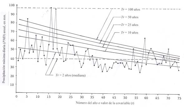
This record was exposed by Katz (2013) as an impressive example of the reduction in the winter (May to October) maximum daily precipitation (MDP) measured at the Manjimup station in the extreme southwest of Australia. The record covers 75 annual values (1930 to 2004), with a declining trend and greater variability at the beginning of the record. Their approximate magnitudes are shown in Table 1, as they were read from a bar graph and are shown in Figure 1.
Table 1 Maximum annual data to be processed for maximum daily precipitation (MDP, in millimeters) and flow (q, m3/s) at the indicated stations.
| Data No. | (MDP) Manjimup station | (q) Aberjona River | (q) Mercer Creek | Data No. | (MDP) Manjimup station | (q) Aberjona River | (q) Mercer Creek |
|---|---|---|---|---|---|---|---|
| 1 | 35.7 | 9.1 | 6.8 | 39 | 34.7 | 18.7 | 5.2 |
| 2 | 49.0 | 5.9 | 5.1 | 40 | 24.8 | 39.6 | 8.9 |
| 3 | 37.8 | 7.4 | 6.7 | 41 | 33.6 | 7.1 | 15.5 |
| 4 | 47.1 | 6.8 | 6.2 | 42 | 24.8 | 9.3 | 17.6 |
| 5 | 84.0 | 5.0 | 5.9 | 43 | 29.9 | 24.4 | 9.1 |
| 6 | 44.9 | 6.2 | 5.4 | 44 | 28.3 | 12.7 | 12.3 |
| 7 | 54.1 | 9.1 | 4.8 | 45 | 34.8 | 22.9 | 11.0 |
| 8 | 45.9 | 9.1 | 4.3 | 16 | 36.1 | 8.5 | 8.6 |
| 9 | 64.8 | 10.2 | 6.4 | 47 | 34.1 | 14.7 | 15.5 |
| 10 | 35.1 | 3.4 | 5.4 | 48 | 34.9 | 24.6 | 18.1 |
| 11 | 52.3 | 7.1 | 5.2 | 49 | 35.0 | 8.8 | 21.3 |
| 12 | 63.9 | 6.8 | 7.2 | 50 | 30.0 | 8.8 | 10.9 |
| 13 | 42.5 | 6.2 | 5.0 | 51 | 35.0 | 19.8 | 13.1 |
| 14 | 31.4 | 7.1 | 7.1 | 52 | 28.1 | 13.9 | - |
| 15 | 54.6 | 13.9 | 5.3 | 53 | 28.0 | 6.8 | - |
| 16 | 97.5 | 19.5 | 5.7 | 54 | 51.5 | 13.9 | - |
| 17 | 49.6 | 10.8 | 11.5 | 55 | 32.1 | 15.0 | - |
| 18 | 95.9 | 4.8 | 6.9 | 56 | 37.0 | 5.9 | - |
| 19 | 50.0 | 11.0 | 9.1 | 57 | 24.1 | 9.1 | - |
| 20 | 42.9 | 4.8 | 9.6 | 58 | 32.0 | 34.0 | - |
| 21 | 51.8 | 5.4 | 7.8 | 59 | 63.7 | 31.1 | - |
| 22 | 35.6 | 6.8 | 7.5 | 60 | 33.3 | 13.3 | - |
| 23 | 37.2 | 10.8 | 11.4 | 61 | 46.3 | 11.0 | - |
| 24 | 57.0 | 22.4 | 13.3 | 62 | 51.8 | 45.3 | - |
| 25 | 53.9 | 6.5 | 14.7 | 63 | 37.9 | 6.8 | - |
| 26 | 54.8 | 8.8 | 11.9 | 64 | 41.2 | 8.8 | - |
| 27 | 43.5 | 2.8 | 19.0 | 65 | 34.1 | 28.3 | - |
| 28 | 47.0 | 10.8 | 17.4 | 66 | 35.0 | 6.5 | - |
| 29 | 36.7 | 18.4 | 11.5 | 67 | 35.0 | 36.8 | - |
| 30 | 29.2 | 13.0 | 10.0 | 68 | 43.4 | 15.3 | - |
| 31 | 34.3 | 21.2 | 23.6 | 69 | 36.0 | 8.2 | - |
| 32 | 48.2 | 4.0 | 14.2 | 70 | 51.4 | - | - |
| 33 | 50.7 | 15.6 | 9.5 | 71 | 30.0 | - | - |
| 34 | 37.6 | 8.5 | 6.5 | 72 | 34.1 | - | - |
| 35 | 42.7 | 7.4 | 18.9 | 73 | 37.0 | - | - |
| 36 | 31.9 | 6.5 | 15.1 | 74 | 36.0 | - | - |
| 37 | 38.8 | 13.0 | 7.8 | 75 | 27.3 | - | - |
| 38 | 29.4 | 10.2 | 7.9 | - | - | - | - |
Series 2: With an upward trend and an increase in variability
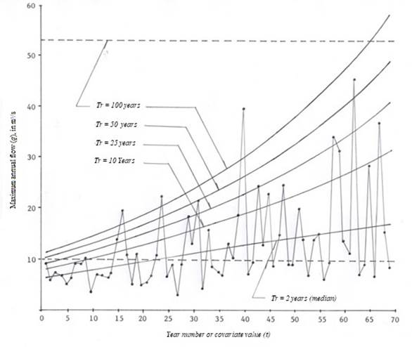
This annual maximum flows record was processed by Vogel et al. (2011), it has 69 values in the period from 1940 to 2008, and comes from a gauging station located on the Aberjona River just after the city of Boston, Massachusetts, USA, so its basin has always been under the increasing impact of urban development. Their approximate values are shown in Table 1, as they were read in a dispersion diagram and are shown in Figure 2.
Series 3: Segment with an upward trend and an increase in variability
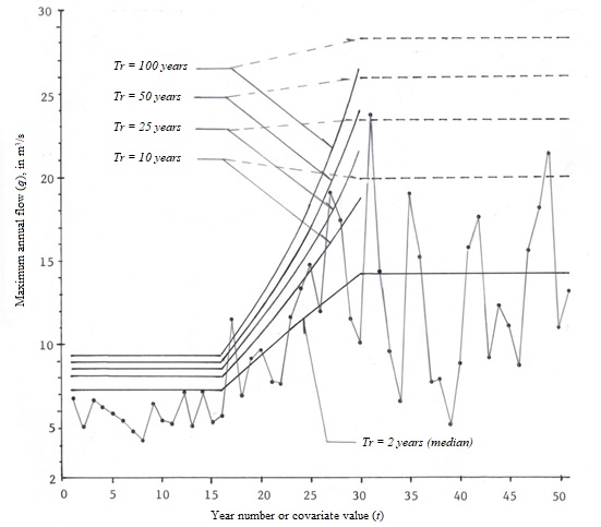
This annual maximum flow record was presented by Gilleland and Katz (2011), and Katz (2013), from a basin in Washington, USA whose Mercer Creek gauging station has 51 values in the period from 1956 to 2006. In the 15-year interval between 1971 and l985, this record was influenced by an increasing and intense urbanization. Because of this, only such a lapse should be considered non-stationary. The approximate data of that series are given in Table 1, as they were read from a bar graph (Katz, 2013) and are shown in Figure 3.
Description of results
Predictions at Manjimup station
The application of equations (22) to (25) to the 75 MDP data in Table 1 led to the following results: μ0 =
Equation (2) using the variable location (Equation (20)) and scale (Equation 18) parameters leads to a standard error of fit (EEA) of 15.5 mm. Table 2 shows some of the predictions within the historical record, and in the future its predictions are not important due to the downward linear trend and the decrease in variability. The predictions with GVE0 stationary model of return periods 2 and 100 years are: 38.7 and 96.6 mm. Figure 1 shows the data and the downward prediction curves.
Table 2 Predictions (mm) in the historical period at the Manjimup station, based on non-stationary GEV11 distribution.
| No. (t) | Year | Data (mm) | Return periods in years | ||||
|---|---|---|---|---|---|---|---|
| 2 | 10 | 25 | 50 | 100 | |||
| 1 | 1930 | 35.7 | 50.9 | 64.4 | 71.8 | 77.6 | 83.5 |
| 10 | 1939 | 35.1 | 48.5 | 60.6 | 67.1 | 72.2 | 77.5 |
| 20 | 1949 | 42.9 | 45.9 | 56.4 | 62.2 | 66.7 | 71.3 |
| 30 | 1959 | 29.2 | 43.2 | 52.5 | 57.5 | 61.5 | 65.5 |
| 40 | 1969 | 24.8 | 40.6 | 48.7 | 53.1 | 56.5 | 60.1 |
| 50 | 1979 | 30.0 | 37.9 | 45.0 | 48.9 | 51.9 | 55.0 |
| 60 | 1989 | 33.3 | 35.2 | 41.4 | 44.8 | 47.5 | 50.2 |
| 70 | 1999 | 51.4 | 32.5 | 37.9 | 40.9 | 43.2 | 45.6 |
| 75 | 2004 | 27.3 | 31.1 | 36.2 | 39.0 | 41.2 | 43.4 |
Predictions on the Aberjona River
The application of equations (22) to (25) to the 69 annual maximum flows (q) in Table 1 led to the following results: μ0 =
Table 3 Predictions (m3/s) in the historical period and in the future at Aberjona River, based on the non-stationary GEV11 distribution.
| No. (t) | Year | Data (m3/s) | Return periods in years | ||||
|---|---|---|---|---|---|---|---|
| 2 | 10 | 25 | 50 | 100 | |||
| 1 | 1940 | 9.1 | 6.1 | 7.9 | 9.1 | 10.1 | 11.3 |
| 10 | 1949 | 3.4 | 7.7 | 10.1 | 11.7 | 13.0 | 14.6 |
| 20 | 1959 | 4.8 | 9.4 | 12.7 | 14.8 | 16.7 | 18.8 |
| 30 | 1969 | 13.0 | 11.1 | 15.6 | 18.5 | 21.0 | 23.8 |
| 40 | 1979 | 39.6 | 12.8 | 18.8 | 22.7 | 26.1 | 29.9 |
| 50 | 1989 | 8.8 | 14.3 | 22.5 | 27.8 | 32.4 | 37.6 |
| 60 | 1999 | 13.3 | 15.7 | 26.8 | 34.0 | 40.2 | 47.2 |
| 69 | 2008 | 8.2 | 16.8 | 31.4 | 40.8 | 49.0 | 58.3 |
| 86 | 2025 | - | 18.4 | 42.7 | 58.6 | 72.4 | 87.9 |
| 111 | 2050 | - | 18.4 | 70.5 | 104.6 | 134.0 | 167.2 |
Predictions at Mercer Creek Station
The application of equations (22) to (25) to the 15 data from 1971 to 1985, i.e., data with numbers 16 to 30 in Table 1, led to the following results: μ0 =
Table 4 shows a portion of the predictions within the historical record and Figure 3 illustrates the data, the upward curves of predictions, and their respective extrapolations.
Table 4 Predictions (m3/s) in the historical period at the Mercer Creek station, based on the non-stationary GEV11 distribution.
| No. (t) | Year | Data (m3/s) | Return periods in years | ||||
|---|---|---|---|---|---|---|---|
| 2 | 10 | 25 | 50 | 100 | |||
| 1 | 1971 | 5.7 | 7.3 | 8.1 | 8.5 | 8.9 | 9.3 |
| 4 | 1974 | 9.1 | 8.9 | 9.9 | 10.6 | 11.2 | 11.8 |
| 7 | 1977 | 7.5 | 10.4 | 12.0 | 13.0 | 13.8 | 14.7 |
| 10 | 1980 | 14.7 | 11.8 | 14.2 | 15.7 | 16.9 | 18.2 |
| 13 | 1983 | 17.4 | 13.3 | 16.7 | 18.9 | 20.7 | 22.7 |
| 15 | 1985 | 10.0 | 14.2 | 18.7 | 21.5 | 23.8 | 26.3 |
For this data series, the predictions with the stationary GEV0 model are of capital importance to approve the extrapolation, toward the beginning and end of the record, of the predictions of GEV11 model that will be the most critical one (Gilleland & Katz, 2011). Therefore, two fittings were made: (1) with the initial stationary record of 15 data (1956-1970) and (2) with the lapse of 21 values (1986-2006) occurring after the trend and increasing variability segment (1971-1985). The predictions of the first fitting were: 5.7, 7.0, 7.6, 7.9, and 8.2 m3/s for the return periods (Tr) of 2, 10, 25, 50, and 100 years, with an EEA = 0.193 m3/s; the predictions for the second fitting were: 12.2, 19.9, 23.4, 25.9 and 28.2 m3/s, with an EEA = 0.691 m3/s.
Then, according to Table 4 results, all predictions of GEV11 are extrapolable toward the start of the record, being greater than those of GEV0. Towards the end of the record, only the median is extrapolated (Tr = 2 years), which is 14.2 m3/s, due to the predictions of the other Tr; those obtained with GEV0 are more extreme than those in the last line of Table 4. The above is shown in Figure 3.
Discussion of results
From a practical point of view, the three numerical applications described cover the common cases in which is applicable the GVE11 model to non-stationary extreme hydrological data records; these are:
1. Series with downward trend and variability, present in records of floods when several small reservoirs have been built within the drainage basin; such behavior may also be associated with global climate change, which was the case with the Manjimup pluviometric station.
2. Records of flows with upward trend, usually associated with basins that have intense urban devel-opment or deforestation, which is the case with Mercer Creek station.
If both processes occur in the basin, or are enhanced by the impacts of climate change, variability also increases toward the end of the sample, which was the case with the Aberjona River.
Predictions, beyond the historical record (t > n), associated with low exceedance probabilities (Design Floods) lack importance in records with downward trend and variability, as they are smaller in the future. The opposite is true for series with upward trend and increasing variability, but in these series it is necessary to explain or account for the probable physical origin of such behavior in order to accept future predictions and try to discern their actual extent. This, because it is extremely risky to accept the behavior of increasing variability, when, for example, it is not known whether urban development will continue in the drainage basin.
To further explain the above, it is indicated that Meylan et al. (2012) have noted that the various approaches or new methods of the FFA, which accept nonstationarity, have generated techniques that allow predictions to be made, associated with low exceedance probability to face the design of hydraulic works. However, there is an urgent need to replace the concept of return periods (Tr, in years), to adapt it to the context of nonstationarity. This is because the Tr is defined with the average recurrence interval, measured over a large number of occurrences. As it happens now, in nonstationarity, mean changes over time, the concept of Tr is meaningless. Details and solutions have been proposed in the references of Sivapalan and Samuel (2009); Salas and Obeysekera (2014); Serinaldi (2015), and Salas, Obeysekera and Vogel (2018).
Conclusions
Flood Frequency Analysis (FFA) in non-stationary records showing non-constant trend and/or variability will be increasingly common in the immediate future, due to increased demand for drinking water and food, as well as to the impacts of climate change and urban development. A simple and uncomplicated computational approach that allows the FFA to be performed on such records is based on the extension of the extreme values theory through the fitting with L-moments, of non-stationary distribution GEV11 with location parameter and scale variables linearly with the time that is entered as covariate. Therefore, GEV11 model is suitable when the series of extreme hydrological data shows trend and increase or decrease in variability that can be accepted as linear.
Based on the results of the three numerical applications in non-stationary records, the simplicity of the above method is observed, as well as the ease of obtaining the predictions associated with non-exceedance probabilities. Graphical contrast is basic for validating the descriptive ability of predictions within the historical record and in the near future. The numerical results of the standard error of fit will allow the contrast and acceptance of other probabilistic non-stationary models. The application of the GEV11 probabilistic model to other extreme hydrological data, such as winds, temperatures, droughts and sea levels, is fully feasible.
Acknowledgements
The corrections suggested by the three anonymous arbitrators A, C and E were appreciated, which allowed the concepts of non-stationary and covariates to be expanded, and the type of method exposed and its advantages to be placed among those available for non-stationary FFA.
REFERENCES
Aissaoui-Fqayeh, I., El-Adlouni, S., Ouarda, T. B. M. J., & St.-Hilaire, A. (2009). Développement du modèle log-normal non-stationnaire et comparaison avec le modèle GEV non-stationnaire. Hydrological Science Journal, 54(6), 141-1156. [ Links ]
Álvarez-Olguín, G., & Escalante-Sandoval, C. A. (2016). Análisis de frecuencias no estacionario de series de lluvia anual. Tecnología y ciencias de agua, 7(1), 71-88. [ Links ]
Benson, M. A. (1962). Plotting positions and economics of engineering planning. Journal of Hydraulics Division, 88(6), 57-71. [ Links ]
Campos-Aranda, D. F. (2003). Capítulo 5: Ajuste de Curvas. En: Introducción a los métodos numéricos: Software en Basic y aplicaciones en hidrología superficial (pp. 93-127). San Luis Potosí, México: Editorial Universitaria Potosina. [ Links ]
Campos-Aranda, D. F. (2018a). Ajuste con momentos L de las distribuciones GVE, LOG y PAG no estacionarias en su parámetro de ubicación, aplicado a datos hidrológicos extremos. Agrociencia, 52(2), 169-189. [ Links ]
Campos-Aranda, D. F. (2018b). Ajuste con momentos L móviles de la distribución GVE con parámetros variables de ubicación y escala. Agrociencia, 52(7), 933-950. [ Links ]
Chow, V. T. (1964). Statistical and probability analysis of hydrologic data. Frequency analysis. In: Chow, V. T. (ed.). Handbook of applied hydrology (pp. 8.1-8.42). New York, USA: McGraw-Hill Book Co. [ Links ]
Clarke, R. T. (1973). Chapter 5: The estimation of floods with given return period. In: Mathematical models in hydrology (pp. 130-146) (Irrigation and Drainage Paper 19). Rome, Italy: FAO. [ Links ]
Coles, S. (2001). Chapter 3: Classical Extreme Value Theory and Models. In: An introduction to statistical modeling of extreme values (pp. 45-73). London, UK: Springer-Verlag. [ Links ]
Cunderlik, J. M., & Burn, D. H. (2003). Non-stationary pooled flood frequency analysis. Journal of Hydrology, 276(1-4), 210-223. [ Links ]
Davis, P. J. (1972). Gamma function and related functions. In: Abramowitz, M., & Stegun, I. A. (eds.). Handbook of mathematical functions (pp. 253-296). New York, USA: Dover Publications. [ Links ]
El-Adlouni, S., Ouarda, T. B. M. J., Zhang, X., Roy, R., & Bobée, B. (2007). Generalized maximum likelihood estimators for the nonstationary generalized extreme value model. Water Resources Research, 43(3), 1-13. [ Links ]
El-Adlouni, S., & Ouarda, T. B. M. J. (2008). Comparaison des méthodes d’estimation des paramètres du modèle GEV non stationnaire. Revue des Sciences de L’Eau, 21(1), 35-50. [ Links ]
Gado, T. A., & Nguyen, V. T. V. (2016). An at-site flood estimation in the context of non-stationarity. I: A simulation study. Journal of Hydrology, 535, 710-721. [ Links ]
Gilleland, E., & Katz, R. W. (2011). New software to analyze how extremes change over time. Eos, 92(2), 13-14. [ Links ]
Hosking, J. R., & Wallis, J. R. (1997). Chapter 2: L-moments. Regional frequency analysis and Appendix: L-moments for some specific distributions. In: An approach based on L-moments (pp. 14-43, 191-209). Cambridge, UK: Cambridge University Press. [ Links ]
Jakob, D. (2013). Non-stationarity in extremes and engineering design. In: AghaKouchak, A., Easterling, D., Hsu, K., Schubert, S., & Sorooshian, S. (eds.). Extremes in a changing climate (pp. 363-417). Dordrecht, The Netherlands: Springer. [ Links ]
Katz, R. W. (2013). Statistical methods for non-stationary extremes. In: AghaKouchak, A., Easterling, D., Hsu, K., Schubert, S., & Sorooshian, S. (eds.). Extremes in a changing climate (pp. 15-37). Dordrecht, The Netherlands: Springer . [ Links ]
Khaliq, M. N., Ouarda, T. B. M. J., Ondo, J. C., Gachon, P., & Bobée, B. (2006). Frequency analysis of a sequence of dependent and/or non-stationary hydro-meteorological observations: A review. Journal of Hydrology, 329(3-4), 534-552. [ Links ]
Kim, S., Nam, W., Ahn, H., Kim, T., & Heo, J. H. (2015). Comparison of nonstationary generalized logistic models based on Monte Carlo simulation. Proceedings of the IAHS (No. 371). (pp. 65-68) 22 June to 2 July, Prague, Czech Republic. [ Links ]
Kite, G. W. (1977). Chapter 12: Comparison of frequency distributions. In: Frequency and risk analyses in hydrology (pp. 156-168). Fort Collins, USA: Water Resources Publications. [ Links ]
López, J., & Francés, F. (2013). Non-stationary flood frequency analysis in continental Spanish rivers, using climate and reservoir indices as external covariates. Hydrology and Earth System Sciences, 17(8), 3189-3203. [ Links ]
López-de-la-Cruz, J., & Francés, F. (2014). La variabilidad climática de baja frecuencia en la modelación no estacionaria de los regímenes de las crecidas en las regiones hidrológicas Sinaloa y Presidio-San Pedro. Tecnología y ciencias del agua, 5(4), 79-101. [ Links ]
Meylan, P., Favre, A. C., & Musy, A. (2012). Chapter 6: Validation of the model. Chapter 9: Perspectives. In: Predictive hydrology. A frequency analysis approach. (pp. 103-117, 161-187). Boca Raton, USA: CRC Press. [ Links ]
Mudersbach, C., & Jensen, J. (2010). Nonstationary extreme value analysis of annual maximum water levels for designing coastal structures on the German North Sea coastline. Journal of Flood Risk Management, 3(1), 52-62. [ Links ]
Papalexiou, S. M., & Koutsoyiannis, D. (2013). Battle of extreme value distributions: A global survey on extreme daily rainfall. Water Resources Research, 49(1), 187-201. [ Links ]
Prosdocimi, I., Kjeldsen, T. R., & Miller, J. D. (2015). Detection and attribution of urbanization effect on flood extremes using nonstationary flood frequency models. Water Resources Research, 51(6), 4244-4262. [ Links ]
Rao, A. R., & Hamed, K. H. (2000). Chapter 7: Extreme Value Distributions. In: Flood frequency analysis (pp. 207-257). Boca Raton, USA: CRC Press . [ Links ]
Salas, J. D., & Obeysekera, J. (2014). Revisiting the concepts of return period and risk for nostationary hydrology extreme events. Journal of Hydrologic Engineering, 19(3), 554-568. [ Links ]
Salas, J. D., Obeysekera, J., & Vogel, R. M. (2018). Techniques for assessing water infrastructure for nonstationary extreme events: A review. Hydrological Sciences Journal, 63(3), 325-352. [ Links ]
Serinaldi, F. (2015). Dismissing return periods! Stochastic Environmental Research and Risk Assessment, 29(4), 1179-1189. [ Links ]
Sivapalan, M., & Samuel, J. M. (2009). Transcending limitations of stationary and the return period: Process-based approach to flood estimation and risk. Hydrological Processes, 23(11), 1671-1675. [ Links ]
Stedinger, J. R. (2017). Chapter 76. Flood frequency analysis. In: Singh, V. P. (ed.). Handbook of applied hydrology, 2nd ed. (pp. 76.1-76.8). New York, USA: McGraw-Hill Education. [ Links ]
Stedinger, J. R., Vogel, R. M., & Foufoula-Georgiou, E. (1993). Frequency analysis of extreme events. In: Maidment, D. R. (ed.). Handbook of Hydrology (pp. 18.1-18.66) New York, USA: McGraw-Hill, Inc. [ Links ]
Vogel, R. M., Yaindl, C., & Walter, M. (2011). Nonstationarity: Flood magnification and recurrence reduction factors in the United States. Journal of the America Water Resources Association, 47(3), 464-474. [ Links ]
Received: August 28, 2019; Accepted: August 11, 2020
 Este es un artículo publicado en acceso abierto bajo una licencia Creative Commons
