


Servicios Personalizados
Revista
Articulo
 texto en
  Inglés (pdf)
 Artículo en XML
 Referencias del artículo
 Enviar artículo por email
Indicadores
-
 Citado por SciELO
 -
 Accesos
Links relacionados
-
 Similares en
SciELO
Similares en
SciELO
Compartir

 Permalink
Tecnología y ciencias del agua
versión On-line ISSN 2007-2422
Tecnol. cienc. agua vol.9 no.5 Jiutepec sep./oct. 2018 Epub 24-Nov-2020
https://doi.org/10.24850/j-tyca-2018-05-07
Articles
Daily precipitation concentration index in the Río Grande de Morelia basin
1Colegio de Postgraduados, Campus Montecillo, Montecillo, Texcoco, Estado de México, México, rodrigo-roblero@hotmail.com
2Colegio de Postgraduados, Campus Montecillo, Montecillo, Texcoco, Estado de México, México, chavezje@colpos.mx
3Universidad Autónoma Chapingo, Chapingo, Estado de México, México, libacas@gmail.com
4Colegio de Postgraduados, Campus Montecillo, Montecillo, Texcoco, Estado de México, México, palacio@colpos.mx
5Colegio de Postgraduados, Campus Montecillo, Montecillo, Texcoco, Estado de México, México, anolasco@colpos.mx
6Colegio de Postgraduados, Campus Montecillo, Montecillo, Texcoco, Estado de México, México, jmgc@colpos.mx
The daily precipitation concentration index (CI) was evaluated as an indicator to characterize the sub-basins in the hydrological basin, which represent different degrees of pluviometric torrentiality. The CI was estimated using the Lorenz curve to evaluate the relative weight of the rainiest days in the series of daily precipitation data, which was recorded in 34 conventional meteorological stations (CWS) in and near the Río Grande de Morelia basin, from its source upstream of the Cointzio Dam, to its mouth in Lake Cuitzeo. The Río Grande passes through the city of Morelia, which has been affected by floods in a cyclical manner, resulting in serious damage: human losses, damage to infrastructure and deterioration in agricultural, livestock and forestry production. A platform was developed in a GIS for the delimitation and characterization of the basin and its 23 sub-basins. The CI for each CWS was calculated, with which isopleths were generated with intervals of 0.01, as well as a raster layer of the CI. The CI average was calculated for the 23 sub-basins and for the basin. Based on the results, a CI torrentiality scale is proposed, such as: Low torrential (0.476-0.515), medium torrential (0.515-0.538), torrential (0.538-0.560) and high torrential (0.560-0.607). Weighted average for the basin resulted in a CI = 0.55, which corresponds to a torrential basin, and the CI was related to the climate of the basin.
Keywords Concentration index; torrentiality; isopleths and basin
Se realizó una evaluación del índice de concentración de precipitación diaria (CI), como un indicador para caracterizar las subcuencas de la cuenca hidrológica, que representan diferentes grados de torrencialidad pluviométrica. El CI se estimó por medio de la curva de Lorenz, para evaluar el peso relativo de los días más lluviosos en series de datos de precipitación diaria, que se registró en 34 estaciones meteorológicas convencionales (EMC), dentro y próximas a la cuenca del Río Grande de Morelia desde su origen, aguas arriba de la presa Cointzio, hasta su desembocadura en el lago de Cuitzeo. El Río Grande pasa por la ciudad de Morelia, la cual se ha visto afectada por inundaciones de forma cíclica, que han dejado como consecuencias graves daños: pérdidas humanas y afectaciones a la infraestructura, así como deterioro en la producción agrícola, pecuaria y forestal. Se elaboró una plataforma en un sistema de información geográfica (SIG), para la delimitación y caracterización de la cuenca, y sus 23 subcuencas. Se calculó el CI para cada EMC, con el que se generaron isopletas con intervalos de 0.01 y una capa ráster del CI; se calculó el promedio del CI para las 23 subcuencas y para la cuenca. Con base en los resultados se propone una escala de torrencialidad del CI, esto es: bajo torrencial (0.476-0.515); medio torrencial (0.515-0.538); torrencial (0.538-0.560), y altamente torrencial (0.560-0.607). El promedio ponderado para la cuenca resultó un CI = 0.55, que corresponde a una cuenca torrencial; el CI se relacionó con el clima de la cuenca.
Palabras clave índice de concentración; torrencialidad; isopletas y cuenca
Introduction
Some hydrological basins and their sub-basins are affected by hydrometeorological events such as extreme precipitations produced by seasonal rains or migratory atmospheric phenomena such as tropical storms and cyclones, among others. These extreme precipitation events create extraordinary runoff that can produce floods, which cause greater damage to human life and urban and hydro-agricultural infrastructure and deterioration of agriculture, fishing and forestry.
For this reason, we proposed that it is possible to evaluate torrentiality in hydrological basins by estimating the Concentration Index (CI). Thus, the objective of this study was to estimate the CI in the sub-basins and basin of the Río Grande de Morelia, Michoacán, Mexico, to assess the degree of torrentiality.
Martín-Vide (2004) proposed a methodology for estimating the Daily Precipitation Concentration Index by applying the Lorenz curve to evaluate the relative weight of the rainiest days in a series of daily precipitation data, recorded in conventional meteorological stations (CWS). Also, Zubieta, Saavedra, Silva and Giráldez (2016) presented a study on the estimation of torrentiality in a hydrological basin using the Concentration Index (CI) and its spatial distribution in the Mantaro River Basin, Peru.
The studies conducted on CI focus on regionalization of precipitation, which is one of the phases to be considered in the study, such as in Martín-Vide and Estrada-Mateu (1992); De Luis, González-Hidalgo and Sánchez (1996); Martín-Vide and Llasat (2000); Martín-Vide (2004); Martín-Vide et al. (2008); Alijani, O’Brien and Yarnal (2008); Zhang, Xu, Gemmer, Chen and Liu (2009); Lana, Burgue, Martínez and Serra (2009); Li, Jiang, Li and Wang (2011); Benhamrouche and Martín-Vide (2011); Vargas, Santos, Cárdenas and Obregón (2011); Velasco-Martínez, Mendoza-Palacios, Campos-Campos and Castillo-Bolainas (2011); Suhaila and Aziz (2012); Cortesi, González-Hidalgo, Brunetti and Martín-Vide (2012); Sarricolea and Martín-Vide (2012); Benhamrouche and Martín-Vide (2012); Zubieta and Saavedra (2013); Espinoza, Herrera and Araya (2013); Shi et al. (2014); Meseguer-Ruiz, Martín-Vide, Olcina-Cantos and Sarricolea-Espinoza (2014); Benhamrouche (2014); Sarricolea and Romero (2015); Benhamrouche et al. (2015); Huang, Huang, Chen, Xing and Leng (2016); Zubieta et al. (2016); Monjo and Martín-Vide (2016); Hamzah, Zainal and Jaafar (2016).
However, in Mexico, no application has been presented using a hydrological approach that allows estimating precipitation torrentiality in hydrological basins using the Daily Precipitation Concentration Index (CI) as an indicator of the degree of aggressiveness or torrentiality of the rain that occurs in the basin and its sub-basins.
In this study, we present the application of the method based on the Daily Precipitation Concentration Index (CI) as an indicator for the estimation of the degree of aggressiveness or torrentiality of a rain event in the hydrological basin and sub-basins of the Río Grande de Morelia, where the city of Morelia is located. The city has been affected cyclically by extraordinary flow of the Río Grande and its tributaries (Conagua, 2016).
Materials and methods
The description of materials includes the location of the study area, the characteristics of the elevation model and information on daily precipitation.
Study area
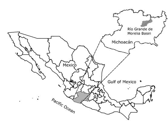
The study was conducted in the Río Grande de Morelia basin, Michoacán, Mexico, where the urban zone of the city of Morelia is located, from upstream of the Cointzio Dam to where the river empties into the Cuitzeo Lake, an area of 1 748 km2 (Figure 1).
Information used
The digital elevation model (DEM) used has a pixel resolution of 15 m and a scale of 1:50 000 (INEGI, 2013).
The meteorological information used is from the National Weather Service’s Conventional Weather Stations (CWS) network (Estaciones Meteorológicas Convencionales del Servicio Meteorological Nacional [SMN, Spanish acronym]). This study included 34 CWS, from which daily precipitation registries from 1923 to 2015 and location were obtained. An average of 0.48% of the data in the series were missing (SMN, 2017).

Delimitation of the hydrological basin
The basins were delimited based on the Continuo de Elevación Mexicano (CEM 3.0) provided by INEGI (2013). The basin of the Rio Grande de Morelia basin was delimited using the extension in the Soil and Water Assessment Tool (Winchell, Srinivasan, Di Luzio, & Arnold, 2013) (Figure 3).
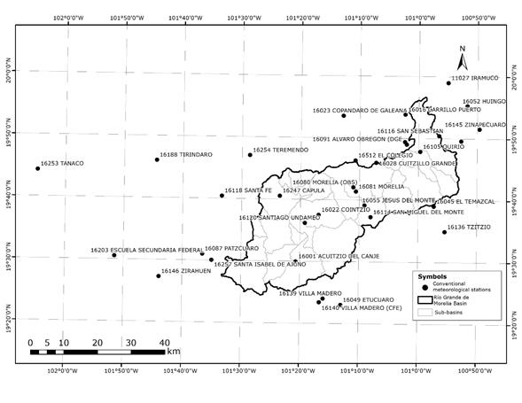
CWS selection, location and georeferencing
The geographic location of each conventional weather station was extracted from the database, using those that are located within and closest to the basin of the Rio Grande de Morelia, as described in Figure 3.
Collection of information on daily precipitation from the CWS registers
The 34 CWSs, their official codes and names, operational condition, georeferencing and length of their registers were identified up to 2015 (SMN, 2017) (Table 1). These CWSs were located in a GIS (Figure 3).
Table 1 General data from the conventional weather stations studied (SMN, 2017).
| Num. | Code | Name | Utm (zone 14N) | Altitude (m) | Years registered | % Missing data | |
|---|---|---|---|---|---|---|---|
| X | Y | ||||||
| 1 | 16001 | Acuitzio del Canje | 253,909 | 2,157,711 | 2 200 | 1961-2008 | 0.37 |
| 2 | 16004 | Álvaro Obregón (Smn) | 287,023 | 2,192,475 | 1 846 | 1964-1986 | 0.05 |
| 3 | 16016 | Carrillo Puerto | 286,636 | 2,201,400 | 1 840 | 1969-2006 | 0.03 |
| 4 | 16022 | Cointzio | 260,775 | 2,171,585 | 2 096 | 1940-2006 | 0.11 |
| 5 | 16023 | Copandaro de Galeana | 268,243 | 2,201,079 | 1 840 | 1969-2001 | 0.01 |
| 6 | 16028 | Cuitzillo Grande | 277,931 | 2,187,050 | 1 987 | 1969-2007 | 0.04 |
| 7 | 16045 | El Temazcal | 295,018 | 2,173,989 | 2 220 | 1965-2014 | 0.06 |
| 8 | 16049 | Etúcuaro | 267,190 | 2,144,739 | 1 690 | 1944-1988 | 0.01 |
| 9 | 16052 | Huingo | 305,078 | 2,203,831 | 1 921 | 1941-2012 | 0.04 |
| 10 | 16055 | Jesús Del Monte | 274,421 | 2,174,360 | 2 180 | 1935-2014 | 0.29 |
| 11 | 16080 | Morelia (Obs) | 271,139 | 2,179,754 | 1 913 | 1986-2014 | 0.07 |
| 12 | 16081 | Morelia | 271,880 | 2,178,484 | 1 908 | 1947-2015 | 0.06 |
| 13 | 16087 | Pátzcuaro | 226,111 | 2,160,051 | 2 140 | 1969-2015 | 0.01 |
| 14 | 16091 | Álvaro Obregón (Dge | 286,508 | 2,193,220 | 1 840 | 1966-2015 | 0.12 |
| 15 | 16096 | Presa Malpaís | 303,216 | 2,193,364 | 1 859 | 1944-2015 | 0.02 |
| 16 | 16105 | Quirio | 291,014 | 2,190,306 | 1 858 | 1963-2015 | 0.11 |
| 17 | 16114 | San Miguel del Monte | 276,184 | 2,170,862 | 1 965 | 1963-2013 | 0.24 |
| 18 | 16116 | San Sebastián | 296 657 | 2 194 976 | 1 836 | 1969-1991 | 0.00 |
| 19 | 16118 | Santa Fe | 232 000 | 2 177 316 | 2 203 | 1963-2014 | 0.04 |
| 20 | 16120 | Santiago Undameo | 256 661 | 2 169 179 | 2 130 | 1953-2007 | 0.03 |
| 21 | 16136 | Tzitzio | 298 196 | 2 166 418 | 1 565 | 1969-2014 | 12.41 |
| 22 | 16139 | Villa Madero | 261 961 | 2 146 652 | 2 097 | 1943-1984 | 0.40 |
| 23 | 16140 | Villa Madero (CFE) | 260 808 | 2 145 560 | 2 182 | 1943-1984 | 0.08 |
| 24 | 16145 | Zinapécuaro | 308 668 | 2 196 872 | 1 880 | 1923-2014 | 0.48 |
| 25 | 16146 | Zirahuén | 213 167 | 2 153 360 | 2 090 | 1947-2014 | 0.03 |
| 26 | 16188 | Tiríndaro | 212 702 | 2 187 987 | 2 002 | 1973-2003 | 0.11 |
| 27 | 16203 | Escuela Secundaria Federal | 199 989 | 2 159 575 | 1 387 | 1975-1982 | 0.05 |
| 28 | 16221 | Fruticultores | 310 023 | 2 198 457 | 1 986 | 1980-2005 | 0.02 |
| 29 | 16247 | Capula | 249 253 | 2 177 280 | 2 097 | 1981-2007 | 0.05 |
| 30 | 16254 | Teremendo | 240 396 | 2 189 406 | 2 188 | 1982-2014 | 0.42 |
| 31 | 16257 | Santa Isabel de Ajuno | 228 855 | 2 158 194 | 2 250 | 1982-1988 | 0.18 |
| 32 | 16512 | El Colegio | 271 796 | 2 187 774 | 1 880 | 1986-2014 | 0.14 |
| 33 | 11027 | Irámuco | 299 457 | 2 210 784 | 1 840 | 1929-1979 | 0.24 |
| 34 | 16253 | Tanaco | 177 252 | 2 185 364 | 2 140 | 1982-2014 | 0.14 |
Station 18145 (Zinapécuaro) contained the longest registry, with 91 years (1923-2014) and station 16257 (Santa Isabel de Ajuno) had the shortest registry, with 6 years (1982-1988).
Calculation of the Lorenz curve
Concentration indexes were determined by calculating and constructing the Lorenz curve as the basis. To calculate the Lorenz curve, Y is the accumulated percentage of precipitation, to which the accumulated percentage of days, X, contributes, where X represents the days that had that precipitation value Martín-Vide, 2004).
Based on this daily precipitation information from each CWS, the following variables are described:
i |
index of the observed daily precipitation value with value Ii, adimensional, i = 1 to NI, number of values defined for the reduced register. |
I i |
Assigned daily precipitation values i, mm. |
F i |
Frequency of daily precipitation that occurs with the value, Ii in the reduced register. |
FA i |
Accumulated frequency of Ni. |
FP i |
Frequency of daily precipitation with which value Ii occurs in the reduced register, %. |
FT |
Total observed frequencies. |
FPi |
Daily precipitation with which value Ii occurs for the reduced register, %. |
PT |
Total observed precipitation. |
Calculation of the Daily Precipitation Concentration Index, CI
Martín-Vide (2004) proposed the concentration index, CI, as an approximation of the numerical representation of differences, shown by the Lorenz curves (Figure 4). In this case, it is used to estimate the importance of rainy days relative to the total accumulated rain in a time series and thereby determine the relative impact of daily precipitation to evaluate the weight of the registered daily maximums relative to the total.
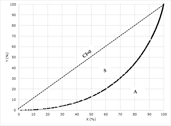
Figure 4 Lorenz curve for the concentration of daily precipitation at the Iramuco Station (1929-1979).
Martín-Vide (2004) associates these curves with exponential type functions:
Where a and b are parameters of the corresponding Lorenz curve.
To determine the values of a and b in the equation, Martín-Vide (2004) obtained the following relationships:
The integral is the area, A, defined by the area under the Lorenz curve between 0 and 100 (Figure 4):
Area, S, is the area under the line of perfect equality (45º) where CI = 0, (100 * 100 / 2 = 5 000) and A is:
The concentration index, CI, is defined as the proportion between S and the area under the line of perfect equality (Figure 4):
The CI are calculated for the 34 conventional weather stations (Table 2 and Figure 5).
Table 2 Calculation of the daily precipitation concentration index and last quartile of the rainiest days at the 34 CWS in the Río Grande de Morelia basin.
| Num. | Code | Name | a | b | A | S | CI | Precipitation (25%) |
|---|---|---|---|---|---|---|---|---|
| 1 | 16001 | Acuitzio del Canje | 0.045 | 0.030 | 1 964.25 | 3 035.75 | 0.607 | 68.29 |
| 2 | 16004 | Álvaro Obregón (SMN) | 0.112 | 0.022 | 2 431.96 | 2 568.04 | 0.514 | 57.68 |
| 3 | 16016 | Carrillo Puerto | 0.135 | 0.020 | 2 385.37 | 2 614.63 | 0.523 | 62.81 |
| 4 | 16022 | Cointzio | 0.096 | 0.023 | 2 349.57 | 2650.44 | 0.530 | 65.32 |
| 5 | 16023 | Copandaro de Galeana | 0.079 | 0.025 | 2 369.12 | 2 630.89 | 0.526 | 60.37 |
| 6 | 16028 | Cuitzillo Grande | 0.067 | 0.027 | 2 304.40 | 2 695.60 | 0.539 | 61.92 |
| 7 | 16045 | El Temazcal | 0.085 | 0.024 | 2 360.11 | 2 639.89 | 0.528 | 59.65 |
| 8 | 16049 | Etúcuaro | 0.082 | 0.025 | 2 410.67 | 2 589.33 | 0.518 | 59.10 |
| 9 | 16052 | Huingo | 0.059 | 0.028 | 2 286.86 | 2 713.14 | 0.543 | 61.30 |
| 10 | 16055 | Jesús del Monte | 0.108 | 0.023 | 2 604.31 | 2 395.69 | 0.479 | 53.86 |
| 11 | 16080 | Morelia (Obs) | 0.033 | 0.034 | 2 022.81 | 2 977.19 | 0.595 | 67.34 |
| 12 | 16081 | Morelia | 0.116 | 0.020 | 2 114.08 | 2 885.92 | 0.577 | 65.48 |
| 13 | 16087 | Pátzcuaro | 0.049 | 0.030 | 2 137.12 | 2 862.89 | 0.573 | 64.09 |
| 14 | 16091 | Álvaro Obregón (Dge) | 0.058 | 0.028 | 2 257.55 | 2 742.45 | 0.548 | 62.75 |
| 15 | 16096 | Presa Malpaís | 0.059 | 0.028 | 2 279.18 | 2 720.82 | 0.544 | 61.52 |
| 16 | 16105 | Quirio | 0.042 | 0.032 | 2 133.01 | 2 866.99 | 0.573 | 64.95 |
| 17 | 16114 | San Miguel del Monte | 0.077 | 0.026 | 2 481.04 | 2 518.96 | 0.504 | 57.18 |
| 18 | 16116 | San Sebastián | 0.061 | 0.028 | 2 272.03 | 2 727.97 | 0.546 | 62.33 |
| 19 | 16118 | Santa Fe | 0.083 | 0.025 | 2 481.03 | 2 518.97 | 0.504 | 55.10 |
| 20 | 16120 | Santiago Undameo | 0.071 | 0.026 | 2 239.28 | 2 760.72 | 0.552 | 63.10 |
| 21 | 16136 | Tzitzio | 0.049 | 0.030 | 2 175.95 | 2 824.05 | 0.565 | 64.88 |
| 22 | 16139 | Villa Madero | 0.064 | 0.028 | 2 319.12 | 2 680.88 | 0.536 | 60.34 |
| 23 | 16140 | Villa Madero (Cfe) | 0.061 | 0.028 | 2 272.03 | 2 727.97 | 0.546 | 60.46 |
| 24 | 16145 | Zinapécuaro | 0.081 | 0.025 | 2 430.13 | 2 569.87 | 0.514 | 57.22 |
| 25 | 16146 | Zirahuén | 0.097 | 0.024 | 2 622.23 | 2 377.78 | 0.476 | 52.44 |
| 26 | 16188 | Tiríndaro | 0.051 | 0.029 | 2 176.01 | 2 823.99 | 0.565 | 64.77 |
| 27 | 16203 | Escuela Secundaria Federal | 0.063 | 0.029 | 2 569.25 | 2 430.75 | 0.486 | 57.44 |
| 28 | 16221 | Fruticultores | 0.044 | 0.032 | 2 375.23 | 2624.77 | 0.525 | 60.62 |
| 29 | 16247 | Capula | 0.061 | 0.028 | 2 312.15 | 2 687.85 | 0.538 | 61.57 |
| 30 | 16254 | Teremendo | 0.093 | 0.024 | 2 501.80 | 2 498.21 | 0.500 | 55.78 |
| 31 | 16257 | Santa Isabel De Ajuno | 0.048 | 0.030 | 2 248.28 | 2 751.72 | 0.550 | 63.70 |
| 32 | 16512 | El Colegio | 0.045 | 0.031 | 2 108.32 | 2 891.68 | 0.578 | 66.15 |
| 33 | 11027 | Irámuco | 0.044 | 0.031 | 2 185.41 | 2 814.59 | 0.563 | 63.53 |
| 34 | 16253 | Tanaco | 0.067 | 0.028 | 2 434.76 | 2 565.24 | 0.513 | 58.26 |
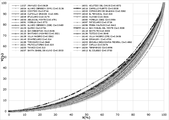
Figure 5 Daily precipitation concentration curves for 34 CWS in the Río Grande de Morelia basin, Michoacán.
Equation 17 was used to calculate precipitation for the last quartile (25%) (Table 3) of rainiest days, Ppd 25% , as a percentage, where:
Table 3 Calculation of the Lorenz curve, Station 11027 (Iramuco), Michoacán, Mexico.
| i | I i | F i | FA i | F i | X i = FAi/FT*100 | P i = I i *F i | PA i | P i | Y i = PA i /PT*100 |
|---|---|---|---|---|---|---|---|---|---|
| mm | Freq. in I i | Freq. Accum in I i | Freq. in I i % | Freq. Accum. in I i % | Prec. in I i mm | Prec. Accum. in I i mm | Prec. in I i % | Prec. Accum. in I i % | |
| 1 | 0.1 | 66 | 66 | 1.72 | 1.72 | 6.6 | 6.6 | 0.02 | 0.02 |
| 2 | 0.2 | 127 | 193 | 3.31 | 5.03 | 25.4 | 32.0 | 0.09 | 0.11 |
| 3 | 0.3 | 75 | 268 | 1.96 | 6.99 | 22.5 | 54.5 | 0.08 | 0.18 |
| 4 | 0.4 | 61 | 329 | 1.59 | 8.58 | 24.4 | 78.9 | 0.08 | 0.26 |
| 5 | 0.5 | 80 | 409 | 2.09 | 10.66 | 40.0 | 118.9 | 0.13 | 0.40 |
| 6 | 0.6 | 27 | 436 | 0.70 | 11.37 | 16.2 | 135.1 | 0.05 | 0.45 |
| … | … | … | … | … | … | … | … | … | … |
| 352 | 60.0 | 1 | 3 833 | 0.03 | 99.92 | 60.0 | 29 598.9 | 0.20 | 99.30 |
| 353 | 65.0 | 1 | 3 834 | 0.03 | 99.95 | 65.0 | 29 663.9 | 0.22 | 99.52 |
| 354 | 65.9 | 1 | 3 835 | 0.03 | 99.97 | 65.90 | 29 729.8 | 0.22 | 99.74 |
| 355 | 77.2 | 1 | 3 836 | 0.03 | 100.00 | 77.20 | 29 807.0 | 0.26 | 100.00 |
| Sum | 3 836 | 1 078 505 | 100.00 | 100.00 |
Results and discussion
The results are presented under the following sub-headings: Calculation of the Lorenz curve for each CWS, calculation of the daily precipitation Concentration Index for each CWS, classification of the sub-basins by the CI, classification of torrentiality according to the CI in the basin and the association between CI and climate.
Calculation of the Lorenz Curve for each CWS
The process is illustrated with daily precipitation data registered at Station 11027 (Iramuco), which began recording on September 1, 1929; the last record was August 31, 1979, and a total of 15 709 data were recorded.
The daily precipitation data were arranged from lowest to highest; data of no precipitation (zero or not available) were excluded. What resulted was a reduced register of Daily Precipitation, Prdr j , in which j = 1 is the minimum value and j = NJ is the maximum.
To estimate the frequency of Prdr j in I i , values were assigned to Ii, namely, I = 1 for its minimum value and I = NI for its maximum value. In this case, I 1 = 0.1 and I NI = 72.2, respectively (355 values). In the reduced register of the station, a value of 0.1 mm of precipitation is presented in 66 days, a value of 0.2 mm occurs 127 days, and so on until reaching a value of 77.2 mm, which occurs only once. The calculation of the Lorenz curve for CWS 11027 (Iramuco) is presented in Table 3 and the curve in Figure 4.
This calculation was performed for the 34 conventional weather stations; each station has its own Lorenz graph (Figure 5).
Figure 5 presents the Lorenz curves for the 34 weather stations. If we analyze the elements of areas A, S and CI, we find that they are the same elements as those presented by Sarricolea and Martín-Vide (2012).
Calculation of the Daily Precipitation Concentration Index, CI, for each CWS
By applying the variables from Equations 16 and 17 for each conventional weather station, we obtain the following results (Table 2).
Parameters a and b varied from a maximum of 0.134 to a minimum of 0.033 and from a maximum of 0.034 to a minimum value of 0.020, respectively. This range of values is also presented by Espinoza et al. (2013), Martín-Vide (2004), and Benhamrouche and Martín-Vide (2012). The values of A ranged from 2 622.2 to 1 964.3, those of S from 3 035.8 to 2 377.8 and of CI from 0.48 to 0.61. If we compare these values with those obtained by Monjo and Martín-Vide (2016), we observe a value of CI = 0.6 for the latitude 19º 42’, presented in world maps and where the region of Morelia, Michoacán, is located. The values of precipitation of 25% of the rainiest days varied from 52.44% to 68.29%.
In the concentration curves, Station 16146 (Zirahuen), with a CI = 0.4756, is the curve that is closest to the line of perfect equality where CI = 0, while Station 16001 (Acuitzio del Canje), with CI = 0.6072, is the farthest from the line, where CI = 1.
The CI was compared with the precipitation of 25% of the rainiest days, and a linear relationship was found (Figure 6).
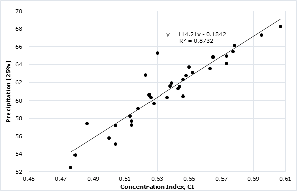
For low CI values (0.476), the percentage of precipitation of the last quartile of the rainiest days is low (52.4%). In contrast, for high CI values (0.607), values of 25% of the rainiest days are high 68.29%. This permits determining torrentiality in a physical sense, since 25% of the rainiest days contributes 68.29% of all the rain registered. Javier Martín-Vide (2004) did this analysis with the CI and 25% of the rainiest days; he found better contrast in regionalization and in data analysis.
Classification of the Sub-basins using CI
First, each sub-basin was delimited. The CI isopleths were then generated, and the CI was calculated by sub-basin.
Delimitation of the Sub-basins
The sub-basins were delimited with the elevation model, using a minimum area of 500 ha; 23 sub-basins resulted (Figure 3).
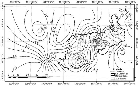
Generation of CI Isopleths
Using the CI results for each conventional weather station, the data were imported in a GIS and a map was constructed by interpolating, in order to obtain the spatial distribution of CI, with a separation of CI = 0.01, with which a raster-type layer of the micro-basins is generated (Figure 7).
Calculation of CI by Sub-basin
With ArcMap (ESRI, 2016) software, the statistical zone tool was used. Input data included the sub-basins layer and the data raster of the interpolated CI grid, and an average value of CI was obtained for each sub-basin (Figure 8).
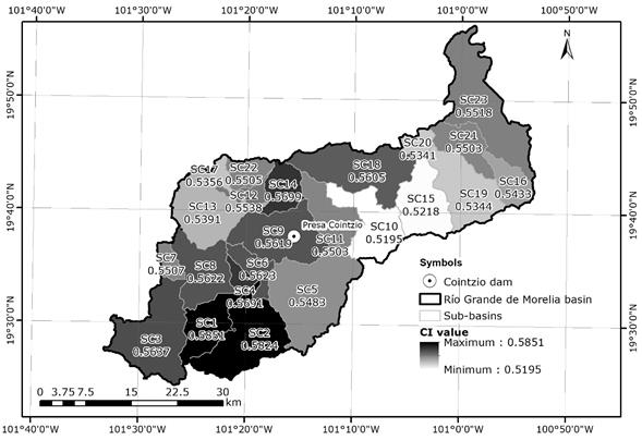
Values in the sub-basins ranged from 0.519 to 0.585. Values in the same range of 0.6 were obtained by Monjo and Martín-Vide (2016). The highest CI values were found in the basins upstream from the Cointzio dam and the lowest near the Río Chiquito micro-basin, which according to the nomenclature used, is basin SC10 (Table 4).
Table 4 CI values by sub-basin for the Río Grande de Morelia Basin.
| Num. | Code | Area (km2) | CI | Level |
|---|---|---|---|---|
| 1 | SC1 | 62.08 | 0.585 | Highly torrential |
| 2 | SC2 | 122.14 | 0.582 | Highly torrential |
| 3 | SC3 | 133.28 | 0.564 | Highly torrential |
| 4 | SC4 | 16.61 | 0.569 | Highly torrential |
| 5 | SC5 | 159.40 | 0.548 | Torrential |
| 6 | SC6 | 28.88 | 0.562 | Highly torrential |
| 7 | SC7 | 17.76 | 0.551 | Torrential |
| 8 | SC8 | 81.77 | 0.562 | Highly torrential |
| 9 | SC9 | 111.09 | 0.562 | Highly torrential |
| 10 | SC10 | 85.52 | 0.520 | Mediumly torrential |
| 11 | SC11 | 61.65 | 0.550 | Torrential |
| 12 | SC12 | 18.09 | 0.554 | Torrential |
| 13 | SC13 | 99.62 | 0.539 | Torrential |
| 14 | SC14 | 43.74 | 0.570 | Highly torrential |
| 15 | SC15 | 80.83 | 0.522 | Mediumly torrential |
| 16 | SC16 | 37.86 | 0.543 | Torrential |
| 17 | SC17 | 74.22 | 0.536 | Mediumly torrential |
| 18 | SC18 | 124.48 | 0.561 | Highly torrential |
| 19 | SC19 | 96.10 | 0.534 | Mediumly torrential |
| 20 | SC20 | 19.01 | 0.534 | Mediumly torrential |
| 21 | SC21 | 50.01 | 0.550 | Torrential |
| 22 | SC22 | 73.82 | 0.551 | Torrential |
| 23 | SC23 | 150.99 | 0.552 | Torrential |
Classification of sub-basin torrentiality by CI
To give the physical context of the CI values in the sub-basins and the basin itself, from the results of the CI values reported in the literature, such as Monjo and Martín-Vide (2016), which range worldwide from 0.38 to 0.87, and those of our study, we propose a manner to compare torrentiality levels within a basin, that is, to determine which is more torrential. Using the concentration index obtained for each sub-basin, a histogram was constructed to identify the distribution of CI in the basin. A normal distribution was obtained, and a normality test (Shapiro Wilks) was applied. The test indicator showed a significant difference of nearly 1; thus, its normal distribution is acceptable and the p-value obtained is higher than the alpha of 0.005 tables. Considering the normality of the data, we propose four levels of torrentiality in the Río Grande de Morelia basin based on the CI value. To this end, we used the quantiles 0% (0.476), 25% (0.515), 50% (0.538), 75% (0.560) and 100% (0.607), which correspond to the boundaries of each class (Table 5).
Table 5 Classification of the concentration index to determine the degree of torrentiality in the Río Grande de Morelia basin.
| Concentration index | Level of torrentiality |
|---|---|
| 0.476-0.515 | Low torrentiality |
| 0.515-0.538 | Medium torrentiality |
| 0.538-0.560 | Torrential |
| 0.560-0.607 | High torrentiality |
The weighted average was calculated for the Río Grande de Morelia basin, obtaining CI = 0.5524; according to the proposed classification, it is of the torrential type.
Association between CI and Climate
To determine the behavior of the sub-basins, it is necessary to relate it to the climate that predominates in the study region. The average CI values in the 23 sub-basins range from 0.5195 to 0.5851. The highest CI values occur in the sub-basins in the upper part of the basin upstream from the Cointzio dam. These sub-basins have a C(E)(w2)(w) climate, which is cool subhumid, the most humid of the subhumid, with summer rains. The months with the highest precipitation are May to October, with more than ten times more rain than the driest month of the year. The percentage of winter rain is < 5% of the annual total; precipitation in the driest month is < 40 mm and mean annual temperature ranges between 5 and 12 º C.
The CI values are between 0.60 and 0.55 in sub-basins downstream from the Cointzio dam, with C(w2)(w) climate type, temperate subhumid, the most humid of the subhumid, with summer rains. The months with the highest rainfall are May to October, when precipitation is at least ten times more than in the driest month of the year. The percentage of winter rain is < 5%, precipitation during the driest month is < 40 mm, with a mean annual temperature that ranges between 12 and 18 ºC.
The lowest CI values, between 0.55 and 0.52, occur in the climate type C(w1)(w), temperate subhumid with medium humidity and summer rains. The highest precipitation occurs from May to October when rainfall is at least ten times that of the driest month of the year. The percentage of winter rain is <5% and precipitation in the driest month is < 40 mm; mean annual temperature ranges between 12 and 18 ºC.
The lowest CI values, between 0.52 and 0.50, are found in the climate type C(w0)(w), which is temperate and less humid than the subhumid climates with summer rains. Rainfall is highest from May to October when it rains at least ten times more than in the driest month of the year. The percentage of winter rain is < 5% and precipitation in the driest month is < 40 mm; mean annual temperature ranges between 12 and 18 º C (INEGI, 2000).
Conclusions
By calculating the daily precipitation concentration index (CI) in the Río Grande de Morelia basin, it is possible to determine the torrentiality level of the rainfall.
By applying this procedure, it is possible to describe how rainfall is distributed across a basin based on geographic information systems.
Immediate applications that can be obtained from this research are identifying the sub-basins that are more torrential than others and proposing basin instrumentation (hydrometric stations).
Given the CI values obtained in this study, we propose a quartile scale to classify the aggressiveness, or torrentiality, of the precipitation in basins and sub-basins in the Río Grande de Morelia basin.
The CI value obtained in the Río Grande de Morelia basin was CI = 0.55, which indicates a torrential type, according to the proposed classification. It is therefore a basin in which extraordinary events can take place and cause flooding in the lower parts, such as those that have been recorded throughout its history and that which occurred in 2015, creating serious problems in the urban area of Morelia (Conagua, 2016).
In the case of the sub-basins, the average CI values in the 23 sub-basins range from 0.52 to 0.59. The highest CI value was found for the sub-basins in the upper part of the basin upstream from the Cointzio dam, which are located in climate types C(E)(w2)(w) cool subhumid and C(w2)(w) temperate subhumid. The lowest CI values are located in climate types C(w1)(w) and C(w0)(w), which are temperate, but in the classification of those that are less sub-humid.
The purpose of this procedure is to have a tool that contributes to the hydrological analysis of basins that are susceptible to flooding, and which can be an indicator of rainfall aggressiveness or torrentiality in basins and tributary sub-basins that in the end results in extraordinary runoff.
Referencias
Alijani, B., O’Brien, J., & Yarnal, B. (2008). Spatial analysis of precipitation intensity and concentration in Iran. Theoretical and Applied Climatology, 94(1-2), 107-124. Recuperado de https://doi.org/10.1007/s00704-007-0344-y [ Links ]
Benhamrouche, A. (2014). Análisis de la concentración diaria de la precipitación en la cuenca del Mediterráneo Occidental. Barcelona, España: Universitat de Barcelona. Recuperado de http://diposit.ub.edu/dspace/bitstream/2445/64206/1/Aziz_Benhamrouche_TESIS.pdf [ Links ]
Benhamrouche, A., Boucherf, D., Hamadache, R., Bendahmane, L., Martin-Vide, J., & Teixeira N., J. (2015). Spatial distribution of the daily precipitation concentration index in Algeria. Natural Hazards and Earth System Sciences, 15, 617-625. Recuperado de https://doi.org/10.5194/nhess-15-617-2015 [ Links ]
Benhamrouche, A., & Martín-Vide, J. (2011). Distribución espacial de la concentración diaria de la precipitación en la provincia de alicante. Investigaciones Geográficas, 56, 113-129. [ Links ]
Benhamrouche, A., & Martín-Vide, J. (2012). Avances metodológicos en el análisis de la concentración diaria de la precipitación en la España peninsular. Anales de Geografia de La Universidad Complutense, 32(1), 11-27. Recuperado de https://doi.org/10.5209/rev-AGUC.2012.v32.n1.39306 [ Links ]
Conagua, Comisión Nacional del Agua. (2016). Actualización y ampliación del estudio control de avenidas en el sistema Río Grande-Río Chiquito y principales drenes, afluentes e incorporaciones de escurrimientos en la ciudad de Morelia y zona conurbada desde la presa de Cointzio hasta su desembocadura. Comisión Nacional del Agua Dirección Local Michoacán. [ Links ]
Cortesi, N., González-Hidalgo, J. C., Brunetti, M., & Martín-Vide, J. (2012). Daily precipitation concentration across Europe 1971-2010. Natural Hazards and Earth System Science, 12, 2799-2810. Recuperado de https://doi.org/10.5194/nhess-12-2799-2012 [ Links ]
De Luis, M., González-Hidalgo, J. C., & Sánchez, J. R. (1996). Análisis de la distribución espacial de la concentración diaria de precipitaciones en el territorio de la Comunidad Valenciana. Cuadernos de Geografía, 59, 47-62. [ Links ]
Espinoza, S. P., Herrera, O. M., & Araya, E. C. (2013). Análisis de la concentración diaria de las precipitaciones en Chile central y su relación con la componente zonal (subtropicalidad) y meridiana (orográfica). Investigaciones Geográficas Chile, 45, 37-50. [ Links ]
ESRI, Environmental Systems Research Institute. (2016). ArcGIS Desktop: Release 10.4. Redlands CA. Environmental Systems Resource Institute. [ Links ]
Hamzah, F. M., Zainal, N., & Jaafar, O. (2016). Daily precipitation concentration index in Bangi, Malaysia. International Journal of Applied Environmental Science, 11(6), 1537-1548. [ Links ]
Huang, S., Huang, Q., Chen, Y., Xing, L., & Leng, G. (2016). Spatial-temporal variation of precipitation concentration and structure in the Wei River Basin, China. Theoretical and Applied Climatology, 125(1-2), 67-77. Recuperado de https://doi.org/10.1007/s00704-015-1496-9 [ Links ]
INEGI, Instituto Nacional de Estadística y Geografía. (2000). Diccionario de Datos Climáticos, Escalas 1:250 000 y 1:1 000 000 (Vectorial). Base de Datos Geográficos. Recuperado de http://www.inegi.org.mx/geo/contenidos/recnat/clima/doc/dd_climaticos_1m_250k.pdf [ Links ]
INEGI, Instituto Nacional de Estadística y Geografía. (2013). Continuo de Elevaciones Mexicano 3.0 (CEM 3.0). Recuperado de http://www.inegi.org.mx/geo/contenidos/datosrelieve/continental/continuoelevaciones.aspx [ Links ]
Lana, X., Burgue, A., Martínez, M. D., & Serra, C. (2009). Una revisión de los análisis estadísticos de las precipitaciones diarias y mensuales en Cataluña. Journal of Weather and Climate of the Western Mediterranean, 6, 15-30. Recuperado de https://doi.org/10.3369/tethys.2009.6.02 [ Links ]
Li, X., Jiang, F., Li, L., & Wang, G. (2011). Spatial and temporal variability of precipitation concentration index, concentration degree and concentration period Xinjiang, China. International Journal of Climatology, 31(11), 1679-1693. Recuperado de https://doi.org/10.1002/joc.2181 [ Links ]
Martín-Vide, J. (2004). Spatial distribution of a daily precipitation concentration index in peninsular Spain. International Journal of Climatology, 24, 959-971. Recuperado de https://doi.org/10.1002/joc.1030 [ Links ]
Martín-Vide, J., & Estrada-Mateu, J. (1992). Diferenciación regional de la España peninsular según la frecuencia relativa de los días con precipitación mayor o igual que 10 milímetros. Papeles de Geografía, 18, 31-38. [ Links ]
Martín-Vide, J., & Llasat, B. M. C. (2000). Las precipitaciones torrenciales en Cataluña. Serie Geográfica, 9, 17-26. Recuperado de https://core.ac.uk/download/pdf/58902370.pdf [ Links ]
Martín-Vide, J., Sánchez-Lorenzo, A., López-Bustins, J. A., Cordobilla, M. J., García-Manuel, A., & Raso, J. M. (2008). Torrential rainfall in northeast of the Iberian Peninsula: Synoptic patterns and WeMO influence. Advances in Science and Research, 2, 99-105. [ Links ]
Meseguer-Ruiz, Ó., Martín-Vide, J., Olcina-Cantos, J., & Sarricolea-Espinoza, P. (2014). La distribución espacial de la fractalidad temporal de la precipitación en la España peninsular y su relación con el Índice de Concentración. Investigación Geográfica Chile, 48, 73-84. [ Links ]
Monjo, R., & Martín-Vide, J. (2016). Daily precipitation concentration around the world according to several indices. International Journal of Climatology, 36, 3828-3838. Recuperado de https://rmets.onlinelibrary.wiley.com/doi/abs/10.1002/joc.4596 [ Links ]
Sarricolea, E. P., & Martín-Vide, J. (2012). Distribución espacial de las precipitaciones diarias en Chile mediante el índice de concentración a resolución de 1 mm, entre 1965-2005. En: Cambio climático, extremos e impactos (pp. 631-639). Salamanca, España: Publicaciones de la Asociación Española de Climatología. [ Links ]
Sarricolea, E. P., & Romero, A. H. (2015). Variabilidad y cambios climáticos observados y esperados en el altiplano del norte de Chile. Revista de Geografia Norte Grande, 62, 169-183. [ Links ]
Shi, P., Qiao, X., Chen, X., Zhou, M., Qu, S., Ma, X., & Zhang, Z. (2014). Spatial distribution and temporal trends in daily and monthly precipitation concentration indices in the upper reaches of the Huai River, China. Stochastic Environmental Research and Risk Assessment, 28(2), 201-212. Recuperado de https://doi.org/10.1007/s00477-013-0740-z [ Links ]
SMN, Servicio Meteorológico Nacional. (2017). Estaciones climatológicas 2016. Recuperado de http://smn.cna.gob.mx/tools/RESOURCES/estacion/EstacionesClimatologicas.kmz [ Links ]
Suhaila, J., & Aziz, J. A. (2012). Spatial analysis of daily rainfall intensity and concentration index in peninsular Malaysia. Theoretical and Applied Climatology, 108(1-2), 235-245. Recuperado de https://doi.org/10.1007/s00704-011-0529-2 [ Links ]
Vargas, A., Santos, A., Cárdenas, E., & Obregón, N. (2011). Análisis de la distribución e interpolación espacial de las lluvias en Bogotá, Colombia. Dyna, 78(167), 151-159. [ Links ]
Velasco-Martínez, L., Mendoza-Palacios, J. de D., Campos-Campos, E., & Castillo-Bolainas, H. (2011). Análisis espacial de las lluvias en la subcuenca del Bajo Grijalva. [ Links ]
Winchell, M., Srinivasan, R., Di Luzio, M., & Arnold, J. (2013). SWAT Help. Texas Agrilife Research. USA: United States Department of Agriculture, Agricultural Reseach Service. [ Links ]
Zhang, Q., Xu, C. Y., Gemmer, M., Chen, Y. D., & Liu, C. (2009). Changing properties of precipitation concentration in the Pearl River basin, China. Stochastic Environmental Research and Risk Assessment, 23, 377-385. Recuperado de https://link.springer.com/article/10.1007/s00477-008-0225-7 [ Links ]
Zubieta, R., & Saavedra, M. (2013). Distribución espacial del índice de concentración de precipitación diaria en los Andes centrales peruanos: valle del río Mantaro. Revista ECIPerú, 9(2), 61-70. [ Links ]
Zubieta, R., Saavedra, M., Silva, Y., & Giráldez, L. (2016). Spatial analysis and temporal trends of daily precipitation concentration in the Mantaro River basin: Central Andes of Peru. Stochastic Environmental Research and Risk Assessment, 31(6), 1305-1308. Recuperado de https://doi.org/10.1007/s00477-016-1235-5 [ Links ]
Received: July 03, 2017; Accepted: March 14, 2018
 Este es un artículo publicado en acceso abierto bajo una licencia
Creative Commons
Este es un artículo publicado en acceso abierto bajo una licencia
Creative Commons
