Introduction

Staple crops are very important not only because they are essential in the diet of Mexicans but also because they are the most important group of crops in Mexican agriculture. They are also the most significant in agricultural imports; in 2024, 46.7 million tons of staple grains and oilseeds were imported, with a value of 17 700 million dollars. A total of 23.6 million tons of corn were imported, along with 5.3 million tons of wheat, 1.03 million tons of rice, and 0.23 million tons of beans, according to Grupo Consultor de Mercados Agrícolas (^{GCMA, 2025}).

All of the above factors affect the income, costs and risk faced by farmers, which has important implications for the national economy, particularly for Mexico’s trade balance and food security: ‘a situation in which all people have physical and economic access to sufficient safe and nutritious food to meet their dietary needs and develop a healthy life’ (^{FAO, 2015}).

Research on cycles, both at the macroeconomic and sectoral levels and by crop group, is vital in the process of defining appropriate and efficient economic policies. According to ^{González-Estrada (2025)}, research on business cycles is essential for understanding the dynamics of Mexico’s agricultural sector and their impact on the economy and food security. In particular, research into cyclical fluctuations in staple crops will allow us to understand the internal and external factors influencing agricultural stability and its risks.

According to ^{González-Estrada et al. (2007)}; ^{Almendra-Arao et al. (2008)}, variations in the production of staple crops are closely related to extreme climate events, volatility in international prices, and changes in production conditions and public policies, especially those that are inconsistent or erroneous.

Studies by authors such as ^{Obstfeld and Rogoff (1996)} indicate that external sector activities are riskier. Crops linked to foreign trade have a higher exposure to risk (^{Komarek et al., 2020}). ^{Díaz-Carreño et al. (2007)} show that production fluctuations follow structured cyclical patterns and show autocorrelation, especially in crops integrated into global markets.

The objectives of this research were: a) to identify the fluctuations in the production of staples crops in Mexico, during the 1993-2022 period, a period corresponding to the liberalization of the country’s foreign trade; b) to analyze cyclical patterns and assess the relationship between the cycles of total gross domestic product (GDP), agricultural GDP, and staple crops, using econometric time series models; and c) to study the underlying risks. The hypotheses were: 1) the production of staple crops has greater volatility than total GDP and agricultural GDP; and 2) the risk of staple crops is greater than the average risk faced by other economic activities.

Materials and methods

Annual data on total GDP, agricultural GDP, and the total production value of the four staple crops in Mexico: corn, beans, rice, and wheat, as well as annual production data, were collected based on ^{SIAP (2022)}; ^{INEGI (2022)}. Statistical analyses were performed in Econometric Views, version 12.

The extraction of the cyclical and growth components was carried out using the method by ^{Hodrick and Prescott (1997)}, widely used in the analysis of macroeconomic time series. According to ^{González-Estrada et al. (2007)}, the method decomposes a time series into two parts: a) the secular or growth trend gt; and b) the cyclical component ct. Thus: yt=gt+ct, for t=1,…,T, where the original time series is yt.

The corresponding nonlinear mathematical programming problem expressed through the Lagrange function is:

s.t: yt=gt+ct.

If L is the lag operator of the observations of a variable, then Lgt=gt-1 and Lmgt=gt-m, m∈Z, and the problem is reformulated as follows:

The first-order condition is: 0=2yt-gt-1+2λ∇2gt+2+2λ∇2gt+1-2+2λ∇2gt1. From this condition, ^{Almendra-Arao and González-Estrada (2008)} obtained the growth and cyclic components, respectively:

According to ^{Hodrick and Prescott (1997)}, if the cyclical component and the second difference of the trend were independently distributed, normal variables with zero mean and variance, σ12 and σ22, respectively, then: λ=σ12σ22. For annual series, λ=100 must be used. The method by ^{Harding and Pagan (2002)} was applied to determine the economic cycles of agricultural GDP and the production value of staple crops in Mexico during the 1993-2022 period (^{INEGI, 2022}); peaks and troughs were previously identified.

An economic cycle is defined as the period between two troughs, including peaks, troughs, expansions, contractions, recoveries and slowdowns (^{Sánchez-Juárez, 2019}). An expansion occurs when GDP increases consecutively for at least two consecutive quarters and exceeds the corresponding value in the secular component of growth. A contraction occurs when GDP declines steadily for at least two consecutive quarters, below its secular trend. The recovery phase is when GDP begins to approach its trend level gradually. In contrast, the slowdown phase occurs when GDP falls below its trend (^{Sánchez-Juárez, 2019}; ^{Schumpeter, 2002}).

According to ^{Harding and Pagan (2002)}, if Ct is the cyclical component for annual data: a) the series of Ct is said to have a peak if it is true that: Ct-1<Ct>Ct+1, and b) the series of Ct is said to have a trough if it is true that: Ct-1>Ct<Ct+1. The censorship rules are: a) the phase, either expansion or contraction, is less than six months; b) the cycles are less than fifteen months; c) if they have consecutive peaks, the highest is selected; and d) if they have consecutive troughs, the lower is chosen.

The New Classical School (NCS) addresses economic fluctuations with the theory of general stochastic dynamic equilibrium of the economy and the theory of real business cycles, unifying the analysis of growth and business cycles (^{González-Estrada, 2018}). Cyclical fluctuations are understood as the co-movements of deviations from the trend in various macroeconomic series. ^{Prescott (1998)}; ^{Kydland and Prescott (1990}, ¹⁹⁸²⁾ highlight the importance of analyzing these co-movements with respect to GDP and its trend. This allows us to identify episodes of volatility and phase change in the economic cycle.

According to ^{Almendra-Arao (2007)}, to obtain the secular trend and its cyclical component, given a time series V: a) the logarithm LV is calculated; b) the ^{Hodrick-Prescott (1997)} filter is applied to LV to obtain the growth component TV; c) the cyclical component is calculated as: DV=LV-TV.

The volatility of a variable yt is the standard deviation of its cyclical component from its secular trend (^{Almendra-Arao and González-Estrada, 2008}). The degree of co-movement of a variable yt with GDP xt is measured by Pearson’s correlation coefficient ρ0, between the cyclical component of the variable yt and the cyclical component of GDP, xt. If ρ0 is positive, zero or negative, the variable is procyclical, acyclical, or countercyclical, respectively.

There is a phase change if the cyclical component of a variable yt changes before, at the same time, or after the cyclical component of GDP and is calculated with Pearson’s correlation coefficients ρj,j∈Z. Where: j represents the lead or lag of the cycle with respect to GDP; if ρj is maximum for a j<0; the cycle is leading; but if j=0; it is coincident and if j>0, it is lagging (^{Agénor et al., 2000}).

Unit root tests are important tools for time series analysis and for determining the stationarity of the series. According to ^{Almendra-Arao et al. (2008)}, a time series is stationary if the mean and autocovariance of the series are not time-dependent; it is integrated of order d and is denoted as Id if, after d operations of differences, the series is stationary. ^{Hamilton (2020}, ¹⁹⁸⁹⁾ reports that the most commonly used unit root tests to investigate the stationarity of a time series are: a) the augmented Dickey-Fuller (ADF) test; b) the Elliott-Rothenberg-Stock (ERS(DF-GLS)) test; c) the Phillips-Perron (PP) test; d) the Kwiatkowski, Phillips, Schmidt, and Shin (KPSS) test; e) the Elliott-Rothenberg-Stock (ERS(OLS)) test; and f) the Ng-Perron (Ng-P) test.

The superior autocorrelation test was the Breusch-Godfrey test, which detected autocorrelation in the residuals of an AR(p) regression model from an ARMA(p, q) (^{Gujarati, 2010}). Let the model be: AR(p): ut=ρ1ut-1+ρ2ut-2+...+ρput-p+εt. The null and alternative hypotheses are: H0: for all i=1,...,p, ρi=0, there is no autocorrelation of any order, and Ha: there is at least one i=1,...,p, ρi≠0, for which there is autocorrelation of some order.

Results and discussion

The cyclical components and the growth of agricultural GDP for the 1993-2022 period were calculated with the method by ^{Hodrick and Prescott (1997)}, with the parameter λ=100. This method was applied to the series expressed in natural logarithms: total GDP, agricultural GDP, production value of staple crops as a whole, and for each. The fluctuating secular trend and the cyclical component of each series were obtained for the 1993-2022 period (Figure 1).

Figure 1 Production value of staple crops and its growth component, 1993-2022. 

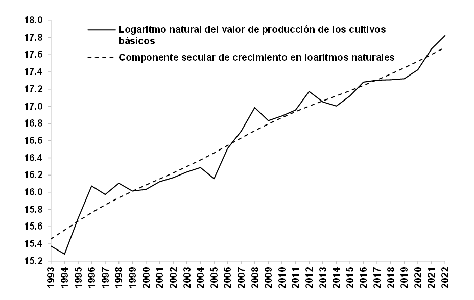
Total GDP exhibited relatively stable growth, whereas agricultural GDP and the production value of staple crops were more volatile, but with a positive long-term trend. The fluctuations in each staple crop are not uniform: corn and wheat have more structured patterns, whereas beans are characterized by high volatility.

In the 1993-2022 period, agricultural GDP showed five trough-to-trough (TT) cycles and five peak-to-peak (PP) cycles. It was in expansion during 70.37% of the time and in contraction during 29.62% of the time. These fluctuations, with average lengths of 4.75 and 5.4 years, respectively, indicate that agricultural GDP gave rise to short cycles. Similarly, morphology tests on the production value of corn, beans, wheat, and rice also identified this type of short cycle.

For the production value of staple crops from 1993 to 2022, three (TT) cycles and five (PP) cycles were identified. It was expanding during 62.96% of the time and contracting during 37.03% of the time. These fluctuations with mean lengths of 7.6 and 7.66 years indicate that the cycles were medium-term or Juglar-type, as can be seen in Figure 2.

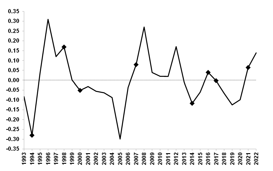
Figure 2 Depressions and peaks, contractions and recoveries in the production value of staple crops in Mexico, 1993-2022. 

Table 1 and 2 show that fluctuations in the production value of staple crops are irregular, have different magnitudes, amplitudes and lengths, but are neither periodic nor symmetrical; this also holds for fluctuations in agricultural GDP and in the production value of crops independently (corn, beans, wheat and rice).

Cycles represent the regularity of fluctuations. The phases of the agricultural cycles and the production value of staple grains in Mexico are irregular: they are neither periodic nor symmetrical. According to ^{González-Estrada and Almendra-Arao (2007)}; ^{Almendra-Arao et al. (2008)}, the same characteristics are observed in the Mexican economy’s economic cycles (Figure 3).

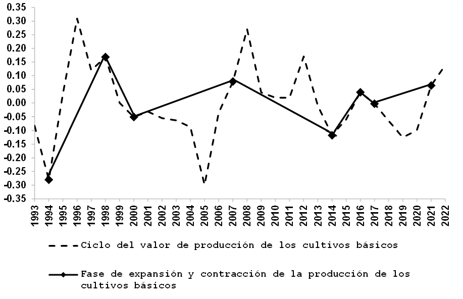
Figure 3 Recoveries, peaks, recessions and depressions in the production value of staple crops in Mexico, 1993-2022. 

The standard deviation of the value of staple crops is 0.1335, and that of agricultural GDP is 0.03, so the production value of staple crops is four times more volatile than agricultural GDP. The standard deviation of corn, beans, wheat, and rice was evaluated in relation to the total production value and contrary to expectations, it was observed that: a) corn is less volatile (0.9844), which makes it the most stable of the staple crops, and b) rice is the most unstable, with a volatility of (1.7909).

Agricultural GDP shows a procyclical relationship with GDP (correlation coefficient (cc)= 0.353). That for the production value of staple crops and agricultural GDP is also procyclical (cc= 0.2572). Nevertheless, the production value of staple crops and GDP have an acyclic relationship (cc= -0.1048). The correlation coefficient between the cycles of the production value of staple crops and of each component: corn, beans, wheat, rice, present positive values and are therefore procyclical. The phase change in the cyclical component of GDP and the production value of staple crops is negative, indicating opposite trends. The agricultural GDP cycle and the production value of staple grains have a positive phase change and move in the same direction (Table 3).

The analyses of the stationarity test of the production value of staple crops and of each crop: corn, beans, wheat and rice, indicate that most of the series are stationary at different confidence levels and that they are integrated variables of order I0. However, in wheat, it is observed that the variable is integrated of order I1.

To analyze the long-term relationship between GDP and agricultural GDP cycles, an ordinary least squares regression was performed, residuals were obtained, an autoregressive process of order four was performed, and the Breusch-Godfrey test was applied. The cointegration vector of the economic GDP and agricultural GDP cycles, calculated based on ^{Engle and Granger (1987)}, is: (1, 0.35757), and the cointegration equation is: cycle of GDP = 0.35757 × cycle of agricultural GDP (Table 4).

Since the value n-pR2>χp2α, H0 is rejected, which indicates serial autocorrelation. Absence of autocorrelation was found between: a) agricultural GDP and staple crops and b) between staple crops.

Conclusions

The production value of staple crops is fluctuating and four times more volatile than agricultural GDP, so the risk costs are higher. There were medium-length cycles in the aggregated production value of staple crops. Fluctuations in the production value of staple crops have a procyclical relationship with agricultural GDP and an acyclical relationship with GDP.

Beans and rice show greater volatility than corn and wheat because they are relatively more influenced by agricultural policies, foreign trade, and climatic conditions. In addition, producers of different staple crops do not face the risk in a homogeneous way, reinforcing the need to design differentiated coverage policies in order to contribute to the country’s food security and economic development.

It was not possible to discuss the above results in the light of other research on the subject, because the present study is unique to Mexico. In addition, another ongoing study is investigating the causes of the fluctuations and cycles investigated here.