SciELO - Scientific Electronic Library Online

 
vol.13 número1Política pública en materia de desarrollo social mediante el Fondo de Infraestructura Social Municipal Potosino índice de autoresíndice de assuntospesquisa de artigos
Home Pagelista alfabética de periódicos  

Serviços Personalizados

Journal

Artigo

Indicadores

Links relacionados

  • Não possue artigos similaresSimilares em SciELO

Compartilhar


EconoQuantum

versão On-line ISSN 2007-9869versão impressa ISSN 1870-6622

EconoQuantum vol.13 no.1 Zapopan Jan./Jun. 2016


Artículos

Ideology, swing voters, and taxation

David Juárez-Luna1 

1Centro de Investigación y Docencia Económicas A. C. Sede Región Centro. Circuito Tecnopolo Norte No. 117, Col. Hacienda Nueva, Aguascalientes, Ags. México. CP 20313. E-mail: david.juarez@cide.edu


Abstract

Ideas about ethnicity, religion, and nationalism among others, which we label “ideology”, seem to affect the preferences of voters, political parties and finally, the equilibrium policy. In this paper we provide a political-economic model that traces the influence of ideology on determining the tax rate in political competition. What we found is that, when the salience of ideology increases, the cohort of voters with the median ideological view become the swing voters. Then, the equilibrium tax rate benefits that cohort of voters.

Keywords: Political economy; Political equilibrium; Ideology; Swing voters

JEL Classification D72; P16

Resumen

Ideas sobre etnicidad, religión y nacionalismo entre otros, que llamamos “ideología”, parecen afectar las preferencias de los votantes, los partidos políticos y, por último, la política de equilibrio. Este artículo provee un modelo político-económico que traza la influencia de la ideología en la determinación de la tasa de impuestos en un ambiente de competencia política. Lo que encontramos es que, cuando la relevancia de la ideología aumenta, el grupo de votantes con la visión ideológica mediana se convierte en los votantes decisivos. Por tal, la tasa de impuestos de equilibrio beneficia a ese grupo de votantes.

Palabras clave: Economía política; equilibrio político; ideología; votantes decisivos

JEL Classification D72; P16

Introduction

In a democracy, as citizens above a certain age have the right to vote, we expect economic policies to be designed to benefit the majority. If the median income is less than the mean, the majority of voters are those whose income is less than the mean. Certainly, even in this situation, economic policy is not always designed to benefit the poor.

Apparently, there are factors, other than the income of the voters, affecting economic policy design. Different ideas about ethnicity, religion, nationalism, views or believes about what is fair, and corruption, among others, which we label “ideology”, affect the preferences of the voters, parties, and finally, the equilibrium policy. The same economic policy, tax rate for instance, could appear to be different for a voter depending on the ideological position of the party that proposes it. The preferences of the voters are defined not just by income as people may also care about ideological positions associated with different political parties (Acemoglu and Robinson, 2006).

In this paper we provide a political-economic model that traces the influence of ideology on determining the tax rate in an economy with political competition. There are two dimensions, a proportional redistributive tax rate and ideology. If a party aligns its preferences to those of the poor, we expect such a party to choose a higher equilibrium tax rate. What we found is that when uncertainty is small, ideology plays an important role on the prevailing economic policy.

The model analyzes decision making in a society consisting of two main social groups: the rich and the poor, both having different preferences on tax rate and ideology. The defining features of the political process are that there are two political parties, each having preferences on tax rate and ideology. Parties offer platforms and voters vote for the platform they like most.2

The main analytical result is that, in equilibrium, if the salience of an ideological issue is high and uncertainty is small, regardless of whether the parties align their preferences to those of the poor or the rich, the cohort of voters with the median ideological position become the swing voters.3 Then, the equilibrium tax rate is designed to benefit that cohort of voters.

This paper is related to the work of Roemer (1998) but is, we believe, richer in its objective and in its approach. We adopt the same framework as his, but we focus on the role of ideology in determining the equilibrium tax rate. We focus on different cases: 1) both parties align their preferences to those of the poor; 2) one party aligns its preferences to those of the poor and the other party to those of the rich and vice versa; 3) both parties align their preferences to those of the rich. Note that as Roemer focuses on the conditions that make the party representing the poor selecting a tax rate less than unity, he only explores case 2.4

The study of ideology and its effect on determining economic policy is not new. In this regard, Dixit and Londregan (1998) model the electoral politics of redistribution when voters and parties care about inequality. They find that in presence of ideological concerns about income redistribution, each party adopt a general proportional income tax, adjusted to appeal to the ideological leanings of groups with disproportionately many “swing” voters. Their results suggest that redistributive politics favours middle classes at the expense of both rich and poor. In the same line, Bénabou (2008) develops a model that focus on ideologies concerning the relative merits of the market versus the state. He takes ideology in two senses of the term: as an exercise in the study of ideas and as the interaction of “subjective mental constructs” across agents and with institutions to generate social cognitions that rest on distorted perceptions of reality. He finds that an equilibrium in which people acknowledge the limitations of interventionism coexists with one in which they remain obstinately blind to them. He also finds that history is important: the interaction among beliefs and institutions generate path-dependent dynamics.

The rest of the paper is organized as follows: Section 2 presents the model. Section 3 computes the equilibrium tax rate. Section 4 offers some further discussion. Section 5 concludes. Appendix contains some technical details not provided in the text.

The model

We examine a jurisdiction with two political parties, two social groups, and a space of voters. The model we shall develop builds on Roemer (1998). Our description begins with the economy.

The economy

We consider a society where the space of citizen traits is ,A=W×R, with generic element (w,a). . The set of income is W=[w_,w¯]R. The set of ideological views is given by the real number line, R.

The population is characterized by a joint probability distribution represented by a density h(w,a)=g(w)r(a|w) on A. Where g(w) is a density on W with mean µ (mean income). For each w, r(a|w) is a density on R. In this economy not all the citizens vote. Suppose that the distribution of voters, that is, of citizens who go to the polls on elections day, is g,(w) where s is a random variable (state) uniformly distributed on [0,1] Let G, be the cumulative distribution function of gs We shall suppose that is strictly decreasing in s.5 Then, in state s, the density of voters is given by:

hsw,a=gs(w)r(a|w) (1)

The interpretation is that while s affects only the wealth distribution of the active electorate, a representative sample of ideological views shows up at each wealth level at the polls in every state of the world.

Policies are given by the pair (t,z) where t is an income tax, and z is the ideological position of the government. The utility function of a citizen with traits (w,a) over policies (t,z) is given by

ux,z;a=1-αx-(α/2)(za)2 (2)

Where x= x(t,w) is net income. The positive number α represents the salience of the ideological issue,α ϵ [0,1].

The political system determines a nonnegative income tax with rate 0 ≤ t ≤ 1 Tax revenues are redistributed via lump sum transfers to all citizens. Assume it is not costly to raise taxes. Then, all the amount collected is redistributed. Given that g(w) is a density on income, per capita taxes collected are t ∫ wg(w)dw=tµ Thus, the net income of a citizen with income w is x(t,w) =(1-t w )w+tµ After substituting this expression into (2), we get the indirect utility function of voter at policy (t,z) which is

vt,z;w,a=1-α1-tw+tμ-(α/2)(z-α)2 (3)

Voting behaviour (Probabilistic voting)

From equation (3), the subsection of voters who prefer policy T 1 =(t 1 ,z 1 ) to policy T 2 =(t 2 ,z 2 ) are those who obtain higher indirect utility with policy T 1 that is: v(t 1 ,z 1 ;w,a) >v(t 2 ,z 2 ;w,a) Such a set, denoted by W(T 1 ,T 2 ) is given by:
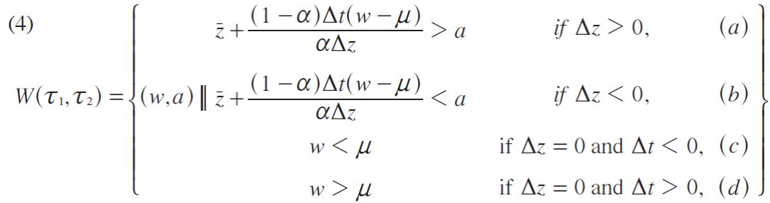
Were Δzz2-z1, tt2-t1 and z¯=(z1+z2)/2

Thus, from equations (1) and (4 (a)), the measure of voters who prefer policy (T 1 ) to policy T 2 if ∆z>0, is given by:

HsWT1, T2=W-Z¯+1-αtw-μαzgs(w)r(a|w)dadw (5)

where H is the cumulative probability distribution with density h s .

Let Φ(z,s) be the cumulative distribution function for ideological views in state s; that is,

We assume: ϕz,s= w-zgswr(a|w)dadw

Assumption (A1) For any z, is Φ(z,s) strictly decreasing in s.6

Policy T 1 defeats policy T 2 in just those states that HSWt1,t2>12. As HSWt1,t2>12 is an event with zero probability, we do not need to worry about it. It follows from A1 and (5) that HSWt1,t2>12 just in case S>S*(T1,T2) where S * (T 1 ,T 2 ) is defined uniquely by:

W-Z¯(1-α)t(w-μ)αzgs*wrawdadw=12 (6)

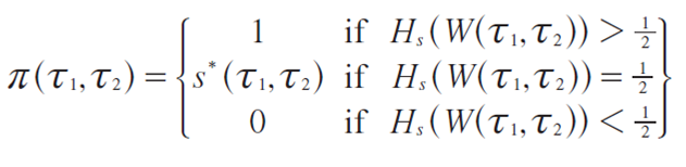
Thus, the probability that policy T 1 defeats policy T 2 is the probability of the event {S<S * } which is S * (T 1 ,T 2 ), since s is uniformly distributed on [0,1]

That is, letting π(T 1 ,T 2 ) be the probability that policy T 1 defeats policy T 2 where Z 2 >Z 1 we have:

(7)

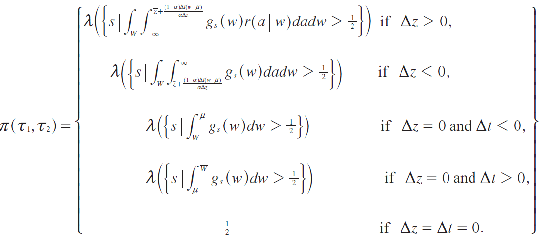
More completely, we may write the function π(T 1 ,T 2 ) for all possible cases, using (4), as follows. Let λ be Lebesgue (uniform) measure on [0,1]. Then:

(8)

Political parties

There are two partisan parties. They have preferences over policies as well as over whether they come to power. Party 1 (P1) aligns its preferences to those of a constituent with traits (w 1 ,a 1 ) while Party 2 (P2) aligns its preferences to those of a constituent with traits (w 2 ,a 2 ) Each party, j, proposes a policy T j =(t J ,z J ) Given a pair of policies (T 1 ,T 2 ) there is only a probability that P1 will win, denoted π(T 1 ,T 2 ) The function π is given by (8) and is known to both parties. Then, the parties’ pay-off functions are

Π1T1, T2=πT1,T2vT1;w1,a1+1-πT1,T2vT2;w1,a1 (9)

Π1T1, T2=πT1,T2vT1;w2,a2+1-πT1,T2v(T2;w2,a2)

The pay-off function of a party in a policy pair is the expected utility of its representative constituent for that pair of policies.7

So far we have defined all the elements of the model. Now we proceed to obtain the equilibrium tax rate.

Political equilibrium

In the case when there is no ideology and all that matters to calculate the tax rate is the income of the voters. If a party aligns its preferences to those of the poor, it chooses the tax rate which is of most benefit to the poor, t¯=1. If the party aligns its preferences to the one of the rich, it, likewise, chooses the best tax rate for them,t¯=0 In the Appendix we also work out this, simpler, one dimensional problem.

Now, we can set the stage for our study. When ideology is included in the preferences, if a party P j aligns its preferences to the ones of the poor, w j , does it choose an equilibrium tax rate of unity to benefit the poor?

Analysis of the Stackelberg equilibrium on taxation and ideology

We compute the equilibrium tax rate when voters and parties alike have preferences over taxation and ideology. Citizens’ preferences are given by (3) while the pay-off functions of the parties are given by (9). We start with case 1, where both parties align their preferences to those of the poor. In the paper we are solving only this case. We include the results for the remaining cases in the next section.8 Then, P1 aligns its preferences to (w 1 ,a 1 ) and P2 to (w 2 ,a 2 ) Where w 1 ,w 2 Parties chose policy platforms to solve the following pair of maximization problems,

P1:MaxΠ1t1,z1T1,T2;α=s*vt1,z1;w1,a1+1-s*v(t2,z2;w1,a1)

P2:MaxΠ2t2,z2T1,T2;α=s*vt1,z1;w2,a2+1-s*v(t2,z2;w2,a2)

Given the two-dimensional nature of the problem, it is difficult to compute the Nash equilibrium. In addition, as we are including ideology in the preferences, we should think of the salience of the parameter α in the utility function as variable, with αϵ[0,1] Then, given the continuity of the payoff functions, for any α there is a Stackelberg equilibrium for the game Ψ a =‹α,(a 1 ,w 1 ),(a 2 ,w 2 ),g,r,{g s },v›

In order to compute the equilibrium tax rate we assume:

Assumption (A2)

  1. In the game Ψ1(i.e., when ux,z;w,a=-12(z-a)2 , there is a finite number of Stackelberg equilibria. For any such equilibrium (z1*,z2*) we have ,and a1<z1*<z2*<a2 and 0<πz1*,z2*<1[/li]

  2. For any equilibrium policy Z2* in Ψ 1, P1’s best response is unique.

  3. For any equilibrium policy Z1* in , Ψ 1, P2’s best response is unique.

Assumption A2 is simply a non-degeneracy axiom about the one-dimensional game Ψ 1 For the analysis of one-dimensional games, which justifies this claim, see Roemer (1999).

Let θ(α) be the Stackelberg equilibrium correspondence, which associates to any of the Stackelberg equilibria of the game Ψ 1 We have the following two facts:

Proposition 3.1 Let A2(b) and A2(c)hold. Then θ(α) is upper-hemi-continuous at .α=1.

Proof: See Appendix.

Let (T 1 (α),T 2 (α)) be a continuum of equilibria for the games Ψ a , α<1 , where T 1 (α)=(t 1 (α), z 1 (α)).

Proposition 3.2 Let A2(a) hold. For sufficiently large α:

  1. zα>0 and zα> is bounded away from 0;

  2. z¯α-a1 is positive and bounded away from zero;

  3. z¯α-a2 is negative and bounded away from zero.

Proof: See Appendix.

We now proceed to calculate the equilibria in our game. Let (z 1 (1),z 2 (1)) be any equilibrium in the game Ψ 1, and ∆z(1)=z 2 (1)-z 1 (1) Let s * be the probability of victory of P1 at this equilibrium. Define the number μ¯=σ¯ρ¯ where σ¯Wwgs*wrz¯1wdw, and ρ¯Wwgs*wrz¯1wdw. By definition μ¯ is the mean income of the cohort of voters with ideological position in the state .Our condition is:

Assumption (A3) For all Stackelberg equilibria in the game , we have:

μ¯-μ>z(1)(μ-w1)2(z11-a1) (10)

(a)

μ¯-μ>z(1)(w2-μ)2(z21-a2)

(b)

Assumption A3 states the conditions for the Stackelberg equilibria to exist in the one-dimensional game Ψ 1. Such conditions focus in the difference in the mean income of the population and the mean income of the cohort of voters with ideological position z¯(1) in the state s * Whether expression (10) holds depends on the value of the right hand side of the inequalities.

Theorem 3.3 Suppose A1, A2, and A3 hold. Then for all sufficiently large α, all Stackelberg equilibria of the game Ψ α have t 1 (α)= t 2 (α)=0

Proof: See Appendix.

Definition 3.4 Let a m (s) be the median ideological view in state s. For any δ>0 we say uncertainty is less than δ if and only if there is a number γ such that, for all s, a m (s) lies in a δ interval around γ.

If uncertainty is sufficiently small, a sufficient condition for the truth of (10) is: the mean income of the cohort of voters with the median ideological view in all states is greater than mean income of the population.

We apply the intuition provided by Roemer (1998) to justify such a condition. If is large, then the game Ψ α is essentially a one-dimensional game on ideology. If uncertainty is small, then the median ideological view varies little across states. In an equilibrium where both parties win with positive probability, both parties must therefore play an ideological position close to the median ideological view. That is, ∆z (1)≈0, as both z 1 (1) and z 2 (1)will be very close to the median ideological view in state s * as will be their average z¯. But since, ∆z (1)≈0, expression (10) is true as long as μ¯>μ.9

We state this result in a corollary for further reference:

Corollary 3.5 For sufficiently small uncertainty, if A1 and A2 hold, the mean income of the cohort of voters with the median ideological view in all states is greater than mean income of the population, and the ideological issue is sufficiently salient, then both parties will propose a zero tax rate in all Stackelberg equilibria.

From Corollary (3.5) we may say that the cohort of the population who hold approximately the median ideological view are the swing voters. If that cohort’s income is greater than the mean population income, then their ideal tax rate is zero. Consequently, competition forces the parties to propose a tax rate of zero, to attract the swing voters. We summarize this result in the following corollary:

Corollary 3.6 Consider a set of tax rates tϵ[0,1] and let preferences be given by (3) as a function of tax rate and ideology. Then, the equilibrium tax rate is given by t * which benefits the cohort of voters with the median ideological view. Those voters are the swing voters.

Further discussion

We have shown that the equilibrium tax rate could be significantly less than unity even if both political parties align their preferences to the ones of the poor (w<µ) In fact, as ideology becomes more important (α increases), the tax rate decreases towards zero. The result gives insight about the role of ideology on determining the equilibrium tax rate.

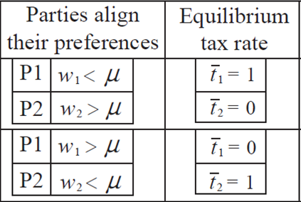
In this paper, we only calculate the equilibrium tax rate for case 1, where both parties align their preferences to those of the poor. Applying the same strategy of analysis used to determine the tax rate in case 1, we now can obtain the equilibrium tax rate for cases 2 and 3. Respectively: 2) one party aligns its preferences to those of the poor and the other party to those of the rich and vice versa; 3) both parties align their preferences to those of the rich. The equilibrium conditions and outcomes are summarized in Table 1.

Source: Own elaboration.

Table 1 Equilibrium conditions and outcomes for the different cases 

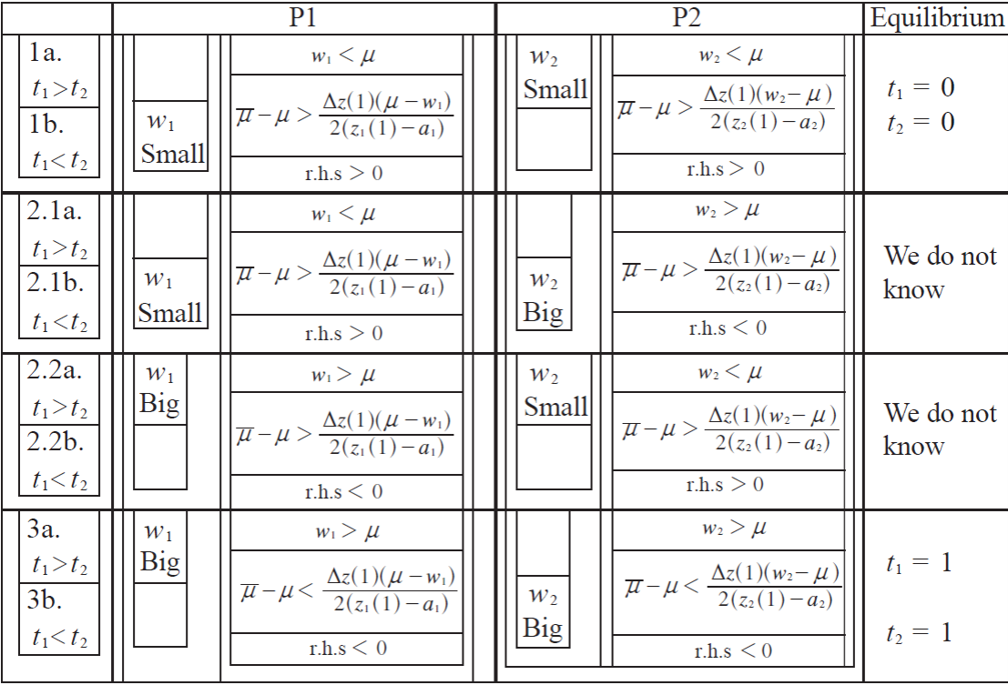
It is difficult to give an equilibrium condition for each of the cases in the table. However, for case 3, when both parties align their preferences to those of the rich, the resulting equilibrium tax rate equals unity,t 1 =t 2 =1. In that case, the key condition turns out to be: a very small uncertainty, and the mean income of the cohort of voters with the median ideological view in all states less than the mean income of the population.

As for case 1, the voters with the median ideological view are the ones benefitting from political competition. The tax rate is designed according to their income regardless of the parties’ preferences. In equilibrium, a political party, P j , proposes a tax rate of unity (t j =1) if the mean income of the cohort of voters with the median ideological view in all states is less than the mean income of the population μ¯<μ.10

The previous analysis strongly depends on the assumption of small uncertainty. If we relax that assumption, the equilibrium ideological positions of the parties are not bounded as the median ideological view could vary a lot across states. In fact, the equilibrium of the one-dimensional game on ideology is (z1*,z2*) where z1* could be considerably different than z2* Such a situation is described by case 2 in the previous table, when it is not possible to obtain the equilibrium tax rate.

Conclusions

Our analysis shows that, even in democracies, where power is apparently given to the majority, ideology plays an important role on the prevailing economic policy. In equilibrium, if the salience of an ideological issue is high and uncertainty is small, regardless of whether the parties align their preferences to those of the poor or rich, the cohort of voters with the median ideological position become the swing voters. Then, the equilibrium tax rate is designed to benefit that cohort of voters.

When uncertainty is high it is not possible to obtain the equilibrium tax rate.

The analysis suggests that, to some extent, the political parties could choose which ideological issues to emphasize with an eye of pushing the electoral debate towards the economic dimension.

References

Acemoglu, D. & Robinson, J. A. (2006). Economic origins of dictatorship and democracy. Cambridge University Press. [ Links ]

Bénabou, R. (2008). Joseph Schumpeter Lecture Ideology, Journal of the European Economic Association, vol. 6(2-3), pp. 321-352. [ Links ]

Dalton, P. D. (2006). Swing voters: understanding late-deciders in late-modernity. Hampton Press. [ Links ]

Dixit, A. & Londregan, J. (1998). Ideology, tactics, and efficiency in redistributive politics, The Quarterly Journal of Economics, MIT Press, vol. 113(2), pages 497-529, May. [ Links ]

Roemer, J. E. (1999). The democratic political economy of progressive income taxation. Econometrica 67 (1999), pp. 1-19. [ Links ]

Roemer, J. E. (1998). Why the poor do not expropriate the rich: an old argument in new garb. Journal of Public Economics, 70, (3), 399-424. [ Links ]

2This approach differs from Roemer (1999), who assumes that parties represent, imperfectly, different constituencies, or economic classes.

3Swing voters tend to be more responsive to policies and as a result the parties will tailor the policies to them (Acemoglu and Robinson, 2006). For a better knowledge of swing voters see Dalton (2006).

4In our paper we find the Stakelberg equilibrium as in Roemer’s analysis, but we do not include the analysis for Roemer’s Party Unanimity Nash Equilibrium (PUNE).

5Following Roemer (1998) we could interpret ‘ S ’ as the weather on the election day. Larger ‘ S ’ means fouler weather. If the weather is foul, fewer poor people turn out to vote; thus G (µ) decreases in S.

6This assumption plays the same role as assuming that G (µ) is decreasing in S. If the rich tend to be more ideological than the poor, and the fraction of rich voters increases with S (as when high S means foul weather in elections day), then A1 surely hold (Roemer, 1998).

7It is generically the case that Nash equilibria in pure strategies, for the game in which the payoff functions are Π 1 and Π 2, do not exist (Roemer, 1998).

8The remaining cases are: 2) one party aligns its preferences to those of the poor and the other party to the ones of the rich and vice versa; 3) both parties align their preferences to those of the rich.

9Forμ¯>μ, the equilibrium policy is[(0,z1*)(0,z2*)]. When z1*<z2* and z1*z2*.

10For μ¯>μ, the equilibrium policy is [(1,z1*)(1,z2*)].When z1*<z2* and z1*z2*.

11Interpretation: ‘s’ is the weather, with larger ‘s’ meaning fouler weather. If the weather is foul, fewer poor voters turn out to vote; thus G (µ) is decreasing in s (Roemer, 1998).

Appendix. Taxation in a one-dimensional context

As an exercise, we find the equilibrium tax rate when the policy space is one-dimensional. In this situation, the party that aligns its preferences to those of the poor (w<µ) proposes a tax rate of unity in the Stackelberg equilibrium. Understanding this exercise should help the reader to maintain their bearings in the more complicated two-dimensional problem explained in the paper.

Assume that the ideological issue is not important then α=0 in equation (3). The indirect utility function of citizen w at tax rate t is:

vt;w=1-tw+tμ=w+t(μ-w) (11)

Now suppose that the distribution of voters, that is, of citizens who go to the polls on elections day, is g s (w), where s is a random variable (state) uniformly distributed on [0,1].

Denote the mean of g s by µ s Let G s be the cumulative distribution function of g s Assume that G s (µ) is strictly decreasing in s.11

Let t 1 >t 2 be two tax policies. It is obvious from (11) that the set of citizens who prefer t 1 to t 2 , denoted W(t1,t2), is:

Wt1,t2={w<μ} (12)

In state s the measure of this set is G s (µ) That is, G s (µ) is the fraction of voters who vote for t 1 over t 2 in state. Now t 1 defeats t 2 just in case it has a majority, i. e., when

Gsμ>12 (13)

As G s (µ) is strictly decreasing in s, (13) is true just in case s<s * , where s * is defined by:

Gsμ=12 (14)

Assuming that there is an s * ϵ(0,1) satisfying (14), then the probability that t 1 defeats t 2 is just s * , since s is uniformly distributed on [0,1].

Now assume the P1 aligns its preferences to those of the poor, w 1 , while P2 aligns its preferences to the ones of the rich w 2 . Then, P1 proposes t 1 , P2 proposes t 2 , and t 1 >t 2 . As P1 wins with probability s * and P2 wins with probability 1- s * , parties’ expected utilities are Π1 (t 1, t 2 ) = s * v(t 1 ;w 2 )+( 1- s * )v(t 2 ;w 2 ) and respectively.

We next compute the Stackelberg equilibrium. Assume that P1 is the ‘incumbent’ and P2 is the ‘challenger’, where by definition, the challenger moves first. A Stackelberg equilibrium exists because the pay-off functions are continuous on the compact set [0,1]2 Let T 2 be P2’s equilibrium policy, and assume T 2 <1 Then P1 obviously maximizes Π1 (t 1, T 2 ) at t 1 =1.

Alternatively, suppose P2 is the incumbent. Let t 1 be any proposal; P2 maximizes Π2 by choosing t 2 =0. Then P1’s problem is to choose t 1 to maximize s * (t 1 ;w 1 )+(1-s * )v(0;w 1 ): the solution is t 1 =1.

Hence, irrespective of whether P1, that is the party that aligns its preferences to the ones of the poor, is the incumbent or challenger, the equilibrium in the game of party competition involves P1 proposing a tax rate of unity. In sum:

Proposition A.1 Let w 1 <µ, let G s * (µ) be strictly decreasing in s, and let u(x)=x be the universal von Neumann-Morgenstern utility function. Suppose there exists s * ϵ(0,1) such that Gs*μ=12. Then, whether the party P1 is the incumbent or challenger, the unique electoral equilibrium in the game of party competition entails T 1 =1 and T 2 =0.

Alternatively, when P1 aligns its preferences to those of the rich w 1 , while P2 aligns its preferences to those of the poor w 2 , then, P1 proposes t 1 and P2 proposes t 2 and t 1 <t 2 . Under such a framework, the equilibrium is such that P1 always proposes a tax rate of zero, regardless of whether it is the incumbent or the challenger. We summarize the equilibrium tax rate in Table 2:

Source: Own elaboration.

Table 2 Equilibrium outcomes in a one-dimensional context 

From the proposition we can conclude that when there is no ideology and the only matter of interest is the income of the voters, if a party aligns its preferences to those of the poor, it chooses a tax rate of unity, T¯=1, to benefice the poor. If the party aligns its preferences to those of the rich, it chooses the best policy for them, t¯=0. Under this situation, we can set the stage for our study. After including ideology in the preferences, will the party P j that aligns its preferences to those of the poor w j , compromise the radical redistributive policy it advocates when only income is the issue?

Proof of important theorems and propositions

Proof of proposition 3.1 Let (T1(α), T2(α)) be a sequence of Stackelberg equilibria in the games Ψ α, and let z 1 (α) and z 2 (α) converge to z 1 (1) and z 2 (1), respectively. Suppose, contrary to the claim, that (z 1 (1), z 2 (1)) is not a Stackelberg equilibrium in Ψ 1. Then,z 1 (1) must not be a best response to z 2 (1); so it must therefore be that there exists an equilibrium pair z1~,z2~ such that z1~ is a best response to z2~ and

Π2z~1,z~2;1>Π2(z11,z21;1)

Let (t1^α,z1^α) be P1’s best response to (t2α,z2~) in Ψ α. Then z1^(1)limαz1^(α) is a best response to z2~ in Ψ 1. By A2b,  z1^1=z1~ . Hence Π2(t1^α,z1^α, t2α,z2~) approaches Π2(z1~,z2~;1) as α approaches 1. In particular, by the above inequality, for large α:

Π2t1^α,z1^α, t2α,z2~>Π2(t1α,z1α,t2α,z2α;α)

This contradicts the fact that (t1α,z1α,t2α,z2α) is a Stackelberg equilibrium in Ψ α, which establishes the claim. It is immediate to do the proof for P1.

By the upper-hemi-continuity of the equilibrium correspondence θ at 1, any converging subsequence of the continuum (T 1 (α), T 2 (α)) converges to an equilibrium of Ψ 1. The claims follow immediately from A2(a).

Proof of proposition 3.2 Let A2(a) hold. For α=1

we have:

a1<z1*<z2*<a2

a1-z1*<0<z2*-z1*<a2-z1*

We end up with

z*>0 (a)

And

a1<z1*<z2*<a2

a1+z2*<z1*+z2*<2z2*<a2+z2*

a1+z2*2<z1*+z2*2<z2*<a2+z2*2

In one side:

0<z2*-a12<z¯*-a1<z2*-a1

then we have:

Z¯*-a1>0 (b)

In the other side:

a1+z2*-2a22<z1*+z2*2-a2<z2*-a2<0

Then we have:

z¯*-a2<0 (c)

Proof of theorem 3.3 First, we are proving that t 1 (α)=0 for the case ∆=t2-t1<0. Suppose to the contrary: that for a sequence of α‘s tending to one, there is a Stackelberg equilibrium of Ψ α in which t 1 (α)>0. We know ∆z(α)>0 by Proposition 3.2; hence, for large α, π(T 1 (α), T 2 (α)) is indeed given by (7), and hence, either π(T 1 (α), T 2 (α))=s * (T 1 (α), T 2 (α)), where s * is defined by (6), or π(T 1 (α), T 2 (α))ϵ{0,1}. But by , since for all equilibria game Ψ 1,πT1α, T2α{0,1} ,it follows that for sufficiently large , , and therefore π(T 1 (α), T 2 (α))=s * (T 1 (α), T 2 (α)).

Differentiating (6) implicitly w.r.t 1 , we may write:

s*t=Wgs*wr(z¯+1-αtw-μαzw)1-αtw-μαzdwW--z¯+1-αtw-μαzs*swrawdadw (15)

as long as the denominator in (15) does not vanish, where we have omitted the argument ‘α’ on the variables z¯ , ∆t and ∆z. But assumption A1 tells us that the expression W--z¯+1-αtw-μαzs*swrawdadw, since this expression is just the derivative of Φ (z,s) w.r.t. s, and so the denominator of (15) does not vanish.

We assume that P1 is the incumbent and P2 is the challenger (i.e., P2 moves first). Since s * is differentiable for large α, so is Π 1 (T 1 ,T 2 ;α) differentiable at (T 1 ,T 2 )= (T 1 (α),T 2 (α)) , for large α. Since T 1 (α) is a best response to T 2 (α), it thereforeδΠ1δz1T1α,T2α,α=0, since z 1 (α) is an interior solution (as the domain of possible z 1 ’s is the real line). This first-order condition can be solved to yield:

Π1τ1,τ2;α=s*vt1,z1;w1,a1+(1-s*)v(t2,z2;w1,a1)

Π1τ1,τ2;α=s*[1-αw1+t1μ-w1-α2(z1-a1)2]+1-s*[1-αw1+t2μ-w1-α2(z2-a1)2]

The F. O. C. subject to is given by:

ðΠ1ðz1=s*-αz1-a1+s*ðz11-αw1+t1μ-w1-α2(z1-a1)2-s*ðz11-αw1+t2μ-w1-α2z2-a12=0

s*z11-αw1+t1μ-w1-α2z1-a12-1-αw1+t2μ-w1+α2(z2-a1)2=s*α(z1-a1)

s*z11-αw1-μt2-t1+α2(z2-a1)2-(z1-a1)2=s*α(z1-a1)

s*z1=s*α(z1-a1)1-αw1-μt2-t1+α2(z2-a1+z1-a1)(z2-a1-z1+a1)

s*z1=s*α(z1-a1)1-αtw1-μ+α(z¯-a1)z (16)

Similarly, it follows that Π1(τ1,τ2;α)t10, since by hypothesis t 1 (α)>0 for all (finite) α.

The just stated inequality can be solved to yield:

ðΠ1ðt1=s*(1-α)(μ-w1)+s*t11-αw1+t1μ-w1-α2(z1-a1)2-s*t11-αw1+t1μ-w1-α2(z2-a1)20

s*t11-αw1+t1μ-w1-α2z1-a12-1-αw1+t2μ-w1+α2z2-a12s*(1-α)(w1-μ)

s*t11-αt1μ-w1-1-αt2μ-w1+α2(z2-a1)2-(z1-a1)2s*(1-α)(w1-μ)

s*t1s*(1-α)(w1-μ)1-αtw1-μ+αz¯-a1-z (17)

an expression whose derivation uses the fact that the denominator of (17) is positive, which follows from Proposition 3.2.

Next, differentiating (6) w.r.t. z 1 yields:

s*z1=-Wgs*wr(z¯+1-αtw-μαz|w)12+(1-α)t(w-μ)α(z)2dwW--z¯+1-αtw-μαzgs*wsra|wdadw (18)

Let the (common) denominator in the fractions on the r.h.s. of (18) and (15) be denoted ‘D’. Using (18) and (16), we can solve for D, eliminating s*z1;

-wgs*wr(z¯+1-αtw-μαz2)dwD=s*α(z1-a1)1-αtw1-μ+α(z¯-a1)z

D=-11-αtw1-μ+αz¯-a1zwgs*wr(z¯+1-αtw-μαz|w)12+(1-α)t(w-μ)α(z)2dws*α(z1-a1)

substituting the expression for D into (15) yields:

s*t1=s*α(z1-a1)wgs*wr(z¯+1-αtw-μαz|w)1-αw-μαzdw1-αtw1-μ+αz¯-a1zwgs*wr(z¯+1-αtw-μαz|w)12+(1-α)t(w-μ)α(z)2dw (19)

In turn, (19) and (17) imply:

s*α(z1-a1)wgs*wr(z¯+1-αtw-μαz|w)1-αw-μαzdw1-αtw1-μ+αz¯-a1zwgs*wr(z¯+1-αtw-μαz|w)12+(1-α)t(w-μ)α(z)2dws*1-αw1-μ1-αtw1-μ+αz¯-a1z ,

(z1-a1)wgs*wr(z¯+1-αtw-μαz|w)μ-wzdwwgs*wr(z¯+1-αtw-μαz|w)12+(1-α)t(w-μ)α(z)2dw(w1-μ)

1z(z1-a1)wgs*wr(z¯+1-αtw-μαz|w)μ-wzdw1α(z)2wgs*wr(z¯+1-αtw-μαz|w)12+(1-α)t(w-μ)α(z)2dw(μ-w1)

αz(z1-a1)wgs*wr(z¯+1-αtw-μαz|w)w-μdwwgs*wr(z¯+1-αtw-μαz|w)12+(1-α)t(w-μ)α(z)2dw(μ-w1) (20)

Letting α→1, (20) becomes, in the limit:

αz(1)(z1-a1)wgs*wr(z¯1|w)(w-μ)dwα(z(1))22wgs*wr(z¯1|w)dw(μ-w1)

2(z11-a1)wgs*wr(z¯1|w)(w-μ)dwwgs*wr(z¯1|w)dw(μ-w1) (21)

Using the definitions of ρ¯,σ¯ and μ¯ provided in the text,

wgs*wr(z¯1|w)(w-μ)dwwgs*wr(z¯1|w)dwz(1)(μ-w1)2(z11-a1)

we can write the negation of (21) as

wgs*wr(z¯1|w)(w-μ)dwwgs*wr(z¯1|w)dw>z(1)(μ-w1)2(z11-a1)

μ¯-μ>z(1)(μ-w1)2(z11-a1) (22)

which is precisely condition (10(a)). Hence, by A3, (21) does not hold, which contradicts the original supposition -that there is a sequence of equilibria at which t ¨1 (α)>0. The reader could verify easily that the inequality in (22) does not change for t 1 =t 2 . Adding the fact that should be small enough to keep 1-αtw1-μ+αz¯-a1z<0 for the case t 1 <t 2 , we get the same expression for (22). Then, if (10) holds and w 1 is small enough, we have t 1 (α)=0 for any case t 1 <t 2, t 1 =t 2, t 1 >t 2 .

Second, we prove that t 2 (α)=0 for the case ∆t= t 2 - t 1 <0.

Suppose to the contrary: that for a sequence of α’s tending to one, there is a Stackelberg equilibrium of Ψ α in which t 2 (α)=0. We know ∆z(α)>0 by Proposition 3.2; therefore, for large α. π(T 1 (α), T 2 (α)) is indeed given by (7), and hence, either π(T 1 (α), T 2 (α))=s * (T 1 (α), T 2 (α)) where s * is defined by (6), or π(T 1 (α), T 2 (α))ϵ{0,1}. But by A2(a), since for all equilibria game Ψt,π{0,1} it follows that for sufficiently large π(T1(α),T2 (α)){0,1}, and therefore π(T 1 (α), T 2 (α))=s * (T 1 (α), T 2 (α)).

Differentiating (6) implicitly w.r.t. , we may write:

s*z2=-Wgs*wr(z¯+1-αtw-μαz|w)1-αtw-μαzdwW--z¯+1-αtw-μαzgs*s(w)ra|wdadw

as long as the denominator in (23) does not vanish, where we have omitted the argument ‘α’ on the variables z¯, t , and z . But assumption A1 tells us that the expression W--z¯+1-αtw-μαzgs*swra|wdadw<0 , since this expression is just the derivative of Φ(z,s)w.r.t. s, and so the denominator of (23) does not vanish.

We assume that P2 is the incumbent and P1 is the challenger (i.e., P1 moves first). Since s * is differentiable for large α, so is Π2(T 1 ,T 2 ) differentiable at (T 1 ,T 2 )= (T 1 (α), T 2 (α)), for large α. Since T 2 (α) is a best response to T 1 (α), it therefore Π2z2(T1α,T2α,α)=0, z 2 (α) since is an interior solution (as the domain of possible z 2 ’s is the real line). This first-order condition can be solved to yield:

Π2τ1,τ2;α=s*vt1,z1;w2,z2+(1-s*)v(t2,z2;w2,a2)

Π2τ1,τ2;α=s*1-αw2+t1μ-w2-α2z1-a22+1-s*1-αw2+t2μ-w2-α2z2-a22

The F. O. C. subject to is given by:

Π2z2=s*z21-αw2+t1μ-w2-α2z1-a22+1-s*-αz2-a2-s*z21-αw2+t2μ-w2-α2z2-a22=0

s*z21-αw2+t1μ-w2-α2z1-a22-1-αw2+t2μ-w2-α2z2-a22=1-s*αz2-a2

s*z21-αt2μ-w2-1-αt2μ-w2+α2z2-a22-z1-a22=1-s*αz2-a2

s*z2=1-s*αz2-a21-αw2-μt2-t1+α2(z2-a2+z1-a2)(z2-a2-z1+a2)

s*z2=1-s*αz2-a21-αtw2-μ+α(z¯-a2)z (24)

Similarly, it follows that Π2τ1,τ2;αt20, since by hypothesis t 2 (α>0) for all (finite) α. The just stated inequality can be solved to yield:

Π2t2=s*t21-αw2+t1μ-w2-α2z1-a22+1-s*(1-α)μ-w2-s*t21-αw2+t2μ-w2-α2z2-a220

s*t21-αw2+t1μ-w2-α2z1-a22-1-αw2+t2μ-w2-α2z2-a221-s*(1-α)w2-μ

s*t21-αt1μ-w2-1-αt2μ-w2+α2z2-a22-z1-a221-s*(1-α)w2-μ

s*z21-s*(1-α)w2-μ1-αtw2-μ+α(z¯-a2)z (25)

an expression whose derivation uses the fact that the denominator of (25) is positive (with w 2 small enough ), which follows from Proposition 3.2.

Next, differentiating (6) w.r.t. z 2 yields:

s*z2=-Wgs*wr(z¯+1-αtw-μαz|w)(12-1-αw-μα(z)2)dwW--z¯+1-αtw-μαzgs*(w)sra|wdadw (26)

Let the (common) denominator in the fractions on the r.h.s. of (26) and (23) be denoted ‘D’. Using (26) and (24), we can solve for D, eliminating s*z2;

-Wgs*wr(z¯+1-αtw-μαz|w)(12-1-αtw-μα(z)2)dwD=1-s*αz2-a21-αtw2-μ+α(z¯-a2)z

D=-1[1-αtw2-μ+α(z¯-a2)z]Wgs*wr(z¯+1-αtw-μαz|w)(12-1-αtw-μα(z)2)dw1-s*αz2-a2

substituting the expression for D into (23) yields:

s*z2=1-s*αz2-a2Wgs*wr(z¯+1-αtw-μαz|w)1-αw-μαzdw[1-αtw2-μ+α(z¯-a2)z]Wgs*wr(z¯+1-αtw-μαz|w)(12-1-αtw-μα(z)2)dw (27)

In turn, (25) and (27) imply:

1-s*αz2-a2Wgs*wr(z¯+1-αtw-μαz|w)1-αw-μαzdw[1-αtw2-μ+α(z¯-a2)z]Wgs*wr(z¯+1-αtw-μαz|w)(12-1-αtw-μα(z)2)dw1-s*αz2-a21-αtw2-μ+α(z¯-a2)z

z2-a2Wgs*wr(z¯+1-αtw-μαz|w)w-μαzdwWgs*wr(z¯+1-αtw-μαz|w)(12-1-αtw-μα(z)2)dw(w2-μ)

1αzz2-a2Wgs*wr(z¯+1-αtw-μαz|w)w-μdw1αz2Wgs*wr(z¯+1-αtw-μαz|w)(αz22-1-αtw-μ)dw(w2-μ)

αzz2-a2Wgs*wr(z¯+1-αtw-μαz|w)w-μdwWgs*wr(z¯+1-αtw-μαz|w)(αz22-1-αtw-μ)dw(w2-μ) (28)

Letting α→1, (28) becomes, in the limit:

αz(1)z21-a2Wgs*wr(z¯+(1)|w)w-μdwαz(1)22Wgs*wr(z¯+1-αtw-μαz|w)dw(w2-μ)

2z21-a2Wgs*wr(z¯+(1)|w)w-μdwz(1)Wgs*wr(z¯+(1)|w)dw(w2-μ) (29)

Using the definitions of ρ¯, σ¯ and μ¯ and provided in the text,

Wgs*wr(z¯+(1)|w)w-μdwWgs*wr(z¯+1-αtw-μαz|w)dwz(1)(w2-μ)2z21-a2

we can write the negation of (29) as

Wgs*wr(z¯+(1)|w)w-μdwWgs*wr(z¯+(1)|w)dw>z(1)(w2-μ)2z21-a2

μ-μ>z(1)(w2-μ)2z21-a2¯ (30)

which is precisely condition (10(b)). Hence, by A3, (29) does not hold, which contradicts the original supposition -that there is a sequence of equilibria at which t 2 (α)>0. The reader could verify easily that the inequality in (30) does not change for the case t 1= t 2 and for the case t 1 <t 2 . Adding the fact that should be small enough to keep 1-αtw2-μ+αz¯-a2z>0 for the case t 1 <t 2 , we get the same expression for (30).

Then, if (10(b)) holds and is small enough, we have at any case t 1 <t 2, t 1 =t 2, t 1 >t 2 and the theorem is proved.

Received: July 07, 2014; Accepted: March 27, 2015

Creative Commons License This is an open-access article distributed under the terms of the Creative Commons Attribution License