nova página do texto(beta)
 Inglês (pdf)
 Artigo em XML
 Referências do artigo
 Enviar este artigo por email
 Citado por SciELO
  Similares em
SciELO
Similares em
SciELO 
 Permalink
Classification JEL: E32, F44, C21.
Introduction
The deceleration of the United States (US) productive activity that started by the end of 2006 derived into the deepest recession the world economy has experienced over the last seven decades. Although its origins can be clearly traced to a single economic activity, the housing sector, and its initial disequilibria and losses were rather modest, its effects spilled over rapidly to the rest of the US financial system. Resulting economic uncertainty and credit cuttings provoked large declines in domestic demand and, eventually, in output, employment, income and investment. Consequently, the US economy entered recession in January 2008 (see Blanchard, 2009; Imbs, 2010).3 The effects of this so-called Great Recession spread quickly to the financial systems of other countries and, eventually, to their real sectors, provoking sharp decreases in their output growth rates (see IMF, 2009, Chapter 1; Blanchard, 2009; Imbs, 2010).
The effects of this crisis transmitted abroad through two major channels. The first was a sharp decline in net capital inflows, especially in the cases of countries with highly integrated financial systems, namely advanced countries, or dependent on external financing, with large external debts, such as several developing countries (Berkmen et al., 2009; Blanchard et al., 2010; Llaudes et al., 2010). The second channel was associated to an abrupt fall of international trade resulting mainly from the deterioration of the external demand of the US and the European Union (EU). As a matter of fact, some authors have argued that this has been the most important transmission channel to emerging market countries, especially to those with large trade ties to the US and EU countries (Blanchard et al., 2010; Bems et al., 2010; Levchenko et al., 2010; Wang, 2010), like Mexico or the Eastern European countries.
Historically, Mexico has been greatly integrated to the US economy both in terms of capital and trade flows, especially after the opening of economy during the eighties (Moreno-Brid y Ros, 2009). The consequences of this process have been multiple but, in economic terms, the high and increasing synchronization of the Mexican business cycles with those of the US has been one of the most significant.4
Hence, the strength the Mexican economy was hit by the decline of the US demand during the recent recession was not surprising at all. Notwithstanding, although generalized, the output effects of the global recession have been heterogeneous across regions. Therefore, the aim of this paper is to analyze the role of structural exposure to external shocks, production specialization and external demand and fiscal shocks link to the Great Recession in explaining the differences in output drops across the Mexican states. Variables measuring these phenomena are incorporated into spatial regression models, which also allow us to give account of possible spillovers of state output falls.
The rest of this paper is organized as follows. In the next explains the transmission of the US recession to the Mexican economy, as well as the economic policy reactions. In section “State recessions” measures and characterizes output drops in the Mexican states, while section “Explaining factors of output drops” defines the model to be estimated and the statistical information to be used. The section “Estimation and results” presents and discusses the main results and, finally, the main conclusions are stated.
Transmission mechanisms, output effects and economic policy in Mexico
The Great Recession started in the US and spilled over the rest of the world through large drops in capital and trade flows. Although several variables defining initial conditions at the beginning of the global recession (such as trade openness, financial integration, fiscal positions, exchange rate regime, current account deficit and leverage, among others) have been mentioned in the literature as significant determinants of output falls, international trade has been identified as one of the most important transmission mechanisms in the case of developing economies (Berkmen et al., 2009; Bems et al., 2010; Levchenko et al., 2010). Indeed, the drop of US total imports, which got a value of 31% from peak to trough,5 affected exports of many other countries, mainly of its major trade partners, like Mexico.
More specifically, although the US gross domestic product (GDP) experienced a mild accumulated percentage decline during the global recession (3.1%), other measures of output exhibited larger falls. For example, industrial and manufacturing production decreased by 17.1 and 20.4%, respectively, while nonagricultural employment had an accumulated drop of 6.2% and the unemployment rate rose by 5.8 percentage points. The combination of all these factors caused a large fall in the US external demand during the last recession affecting the exports of its trade partners.
Then, given the high and increasing integration of the Mexican economy to the US economic dynamics, the flows of external resources to the former declined severely. Exports, FDI, remittances, incomes from tourism and the number of tourists had accumulated drops of 31.9, 68.2, 25.5, 26.1 and 28.7%, respectively. This information can support not only the view that the Great Recession can be seen as an external demand shock to the Mexican economy, but also it can clarify the role of these variables as the relevant transmission mechanisms. Furthermore, given the high synchronization of the business cycles of both economies (Ramírez and Castillo, 2009; Mejía and Campos, 2011) and the magnitude of their international transactions, as well as their relative sizes, the strong impact of the Great Recession on the Mexican economy was not surprising at all. Thus, its GDP had an accumulated growth rate of -9.4% between 2008.2 and 2009.2, whilst the corresponding figures of the industrial and manufacturing production equated -17.0 and -22.0%, respectively, between February 2008 and May 2009.
Now, the shares in GDP of external resources suggest that trade may have acted as the main transmission channel of this recession and also as one of the most important determinant of state output drop. Indeed, over the period 2003-2009, exports represented 27.3% of GDP, which contrasts with the fact that FDI, remittances and incomes from tourism only got 2.4, 2.6 and 1.4%, respectively. Hence, although these variables could have had significant effects on the local level, they played a rather limited role from a macroeconomic perspective. Next, we explore the role of these variables in explaining output falls at a state level.
State recessions
The effects of the Great Recession on output have been negative and heterogeneous across the Mexican states. In this paper, state output drops are measured as the accumulated growth from the peak preceding the recession up to the trough defining its end.6 Output, in turn, is measured by the Quarterly Indicator of the State Economic Activity (QISEA) published by the National Institute of Statistics and Geography (INEGI) of Mexico. In order to have a more complete picture of the Great Recession effects, we analyze both total and sector (industrial and services) QISEA.7 The analysis period corresponds to that of the Great Recession and it starts in 2007 and ends in 2009 in most cases, although in some others it begins before and ends later, depending on the dates identifying the specific recession of each state and sector (see Appendix 1).
Graph 1 shows total and sector output drops in the Mexican states. In principle, some remarkable patterns can be identified. First, output drops were larger in the industrial production sector, especially in the states of Coahuila, Tamaulipas and Sonora, with accumulated growth rates of -25% or less. These states are located in the northern border of Mexico and are highly related to ‘maquila’ production. Also, output experienced large falls in states where transportation equipment represents a large share in its total production, like Puebla. On the other hand, it is rather odd that states without a significant international integration, such as Michoacán and Nayarit, have also experienced large output declines. On the other extreme, due to the increase in international oil prices, Tabasco, a major producer of this good, presented a growth of 8.2% over the national recession period.8 Second, output of the services sector experienced a generalized decline, especially in the case of Quintana Roo, a state specialized in touristic services. Third, the combination of severe falls in output both in the industrial and services sectors yielded considerable falls in total output in most states, especially in Baja California, Tamaulipas, Nuevo León, Colima, Aguascalientes, Querétaro, Puebla, Hidalgo, Guerrero and Chiapas.
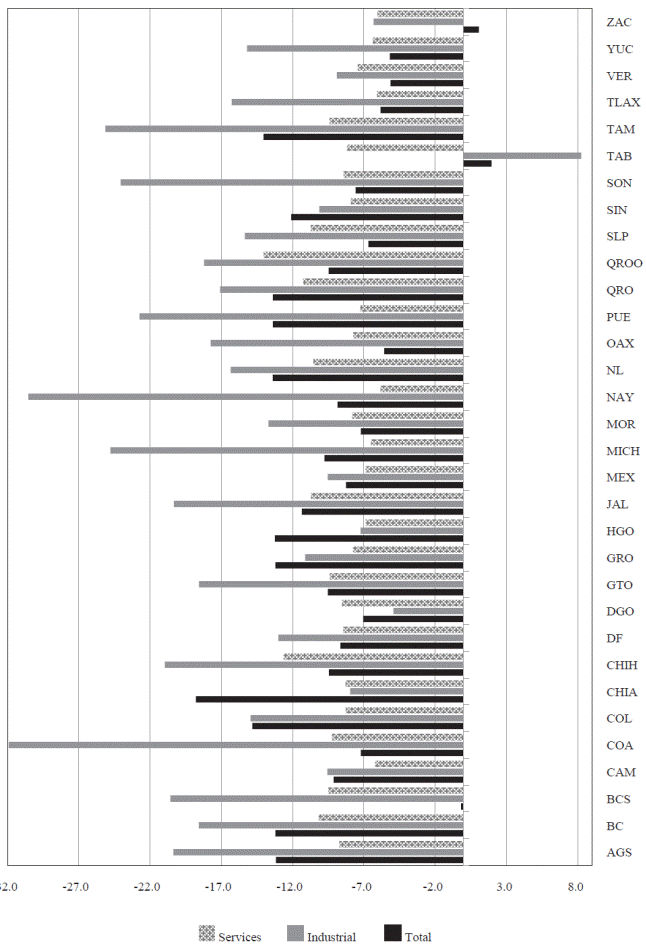
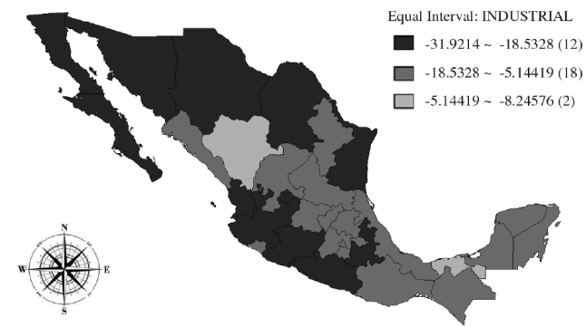
The spatial distribution of output drops is presented in Maps 1 to 3. The former shows that falls of industrial production have been larger in the northern bordering states (mainly Sonora, Coahuila and Tamaulipas) and in the center-West region (especially in Jalisco and Nayarit) as well as in some central states that could have been affected by the huge decrease in the industrial output of Puebla. It is worthwhile to underline that accumulated falls of output in this sector range from -2 to -22 per cent in 25 out of 32 states, which indicates a large variability in the performance of industrial output over the Great Recession across the states. Also, it can be seen that six states, located in the central, West-central and northern regions, outstand with accumulated falls that exceeded 21%.
Source: Own elaboration based on data from INEGI (2012).
Map 1 Output falls in Mexican states industrial production over the Great Recession
Source: Own elaboration based on data from INEGI (2012).
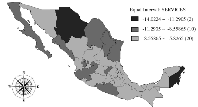
Map 2 Output falls in Mexican states services production over the Great Recession
Source: Own elaboration based on data from INEGI (2012).
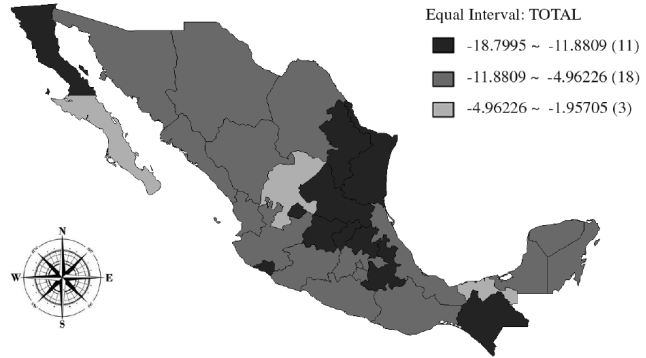
Map 3 Output falls in Mexican states total production over the Great Recession
In turn, Map 2 illustrates how the output of the services sector experienced larger drops in the West-central and northern regions. Notice that, in this case, the growth rates ranged from around -12.0% to -5.8%, which suggests that although generalized across the states output falls were more homogeneous within this sector. In principle, these declines in output may be explained by the transmission of external shocks from the manufacturing production to the services sector through activities such as the transport, storage, distribution and sales of goods.
Finally, it can be observed in Map 3 that total output drops have been larger in the northern states, which results not surprising given the high degree of integration of their productive processes to those of the US firms. Also, it is interesting to notice that western states exhibited significant drops that may have resulted from the transmission of external shocks from manufacturing to other sectors. We must highlight that the accumulated growth rates of most states in the country lie between -3.0 and -13.0 percent, which clearly indicates the occurrence of generalized deep recessions.
Next, according to the objective of this paper, we explore the existence of (spatial) dependence in the magnitudes of the state output falls. In other words, we analyze the possibility that this variable can be determined not only by factors of the same area, but also by phenomena belongings to neighboring areas. If such is the case, there would be evidence of spatial autocorrelation, which refers to the absence of independence between the observations of a cross-section data set (Anselin, 2005; LeSage and Pace, 2009). More specifically, when locations with high (low) levels of one variable are surrounded by locations with also high (low) levels of the same variable it is said that there exists positive spatial autocorrelation. On the contrary, if locations with high (low) levels of one variable are neighbors of locations with low (high) levels of the same variable, then there is evidence of negative spatial autocorrelation.
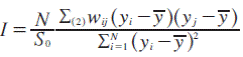
As it is very well known, global spatial autocorrelation can be computed by using the Moran´s I index, which measures the degree of linear association between a vector of observed values and the weighted average of the corresponding values of the neighboring locations for a particular observation. The null hypothesis assessed in this exercise is that there is no spatial autocorrelation and the corresponding test statistic follows a standardized normal distribution (see Appendix 2 for details).
The computations of the Moran´s I index yielded the following test statistics (p-values) for total, industrial and services production: -0.297 (0.009), 0.035 (0.279) and -0.056 (0.440), respectively. These results imply that there is evidence of spatial and negative autocorrelation only in the case of total production. Additional evaluation of this property is carried out in the next section in the context of spatial regressions.
Explaining factors of output drops
The Mexican states output drops experienced during the Great Recession can be explained by multiple factors. On the basis of theoretical models and international empirical evidence, aforementioned, and accepting that the recession in Mexico can be seen as a consequence of exogenous demand shocks, the explanatory variables can be organized in three different sets measuring structural exposure to external shocks (initial conditions), specialization in tradable goods, and external demand and fiscal shocks directly linked to the Great Recession.9
Hence, the first set relates to the importance in the state economic activity of the international flows of goods and capital that allows us not only measuring the degree of integration of the Mexican states to the global economy, but its sensitivity to external shocks as well. The second set refers to the share in state output of the production of tradable goods, especially of durable goods,10 whose cyclical fluctuations also result to be highly synchronized to the US business cycle. Finally, the third set contains variables associated to the transmission of the Great Recession from the US to the Mexican economy through international transactions as well as to the fiscal policies instrumented by the federal and state governments to mitigate its negative effects (Villagómez and Navarro, 2010). Specifically, the model explaining output drops in the Mexican states can be expressed as follows:
 (1)
(1)
where y denotes a n x 1 vector containing the observation of output drops, X i (for i = 1, 2, 3) denotes a n x k i matrix of explanatory variables, with associated parameters contained in the k i x 1 vector b i , and u represents the disturbance vector of order n x 1, with a null vector mean 0 and a variance-covariance matrix σ 2 I, that is u ~ iidN (0,σ 2 I). The specific variables contained in matrices X i are as follows: X 1 = [REM, X, FDI, TOUR, MAN], X 2 = [MAQ, ESP i ] and X 3 = [TREM, TFDI, TG i ], where REM, X, FDI, TOUR and MAN denote the share in state GDP of remittances, exports, foreign direct investment, tourism and manufacturing production; notice that exports are also measured as the share of the basic sector in GDP (BAS).11MAQ stands for the ratio of ‘maquila’ to manufacturing production, while ESP i denotes different specialization variables such as the share in manufacturing production of the transportation equipment production (AUT), as well as different combinations of the production of textiles (sector 2), chemicals (sector 5) and metallic products and machinery and equipment (sector 8), denoted as R258, R28 and R58. 12 In matrix X 3 , the prefix “T” denotes the growth rate of the corresponding variable. Finally, G i denotes government expenditure, as measured by the net federal expenditure (NFE), net state expenditure (NSE) and federal fix investment by state (FFIS). Further details of the data set are given in appendix 3.
Now, eight different specification models are defined depending of the use of alternative variables to measure exports and specialization. The first four specifications include X whilst the latter do so with BAS. In turn, AUT, R28, R58 and R258 define four models in each case giving a total of eight.
In addition, model (1) has been extended in order to incorporate the effects of space in the dynamics of output drops. On the basis of the corresponding statistic tests (presented below), spatial autoregressive models are the most appropriated.13 Then, formally, the general model can be specified as:
 (2)
(2)
where W is the row-standardized spatial weight matrix with entries equal to 1 if the states share a border and 0 otherwise; therefore, Wy is the spatial lag of the endogenous variable, ρ is the spatial autoregressive coefficient which reflects the intensity of interdependencies between the sample observations, and u is the random variable that follows a white noise process.
Estimation and results
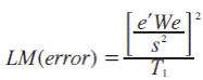
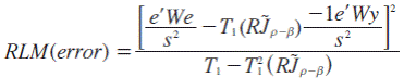
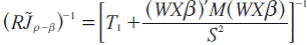
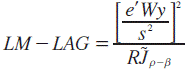
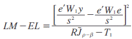
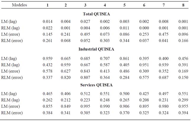
Model (2) is used to explain output drops in the Mexican states as a function of the explanatory variables defined in expression (1). Then, following Anselin (2005), this model has been chosen on the basis of the Lagrange multiplier (LM) tests defined in Appendix 2. The estimated p-values of the statistics LM(lag) and LM(error) to evaluate the null of no spatial autocorrelation between the dependent variable (substantive autocorrelation) and the residuals (residual autocorrelation) in the regression model (1), estimated by ordinary least squares, are presented in Table 1. The set of statistic tests also includes versions robust to misspecifications, which are denoted as RLM(lag) and RLM(error), respectively.
Table 1 p values of the LM tests to choose between lag or spatial error models
Source: Own elaboration.
In the case of total QISEA, the estimated p-values of the LM(lag) test statistic allow us to reject the null at least at 5% of significance for all specifications, while the estimates corresponding to the LM(error) statistic allow us to do so only at 10% in the case of specifications 4, 5 and 8. However, since the estimated p-values of the LM(lag) statistics are lower than those of the RLM(error) statistics, we decided to estimate lag regression models for the whole set of specifications.14 In turn, notice that the estimated LM test statistics provide support to the null hypothesis of no autocorrelation for all model specifications in the cases of industrial and services QISEA. Altogether, this evidence is consistent with that provided by the Moran´s I index. Thus, there seems to be spatial autocorrelation only in the case of total QISEA. Consequently, the econometric analysis is based on model (2) for total QISEA and model (1) for industrial and services QISEA. The final specification of each model was obtained following a “general to specific approach”: essentially, models defined in (1) and (2) are estimated and then the least significant variable is dropped out and the model is estimated again. The process continues up to the point when all variables are statistically significant at least at a 10% level of significance.
The results for the industrial and services production are shown in Tables 2 and 3. As it can be seen, the estimated models explain over 55% of the output drops variability, as measured by the determination coefficient R 2 .15 It is worth underlining that the estimates of the parameters are largely robust both in terms of value and sign. In general, the exposure variables have the negative expected sign suggesting that the higher the exposition to external shocks the greater the fall in output.
Table 2 Estimation results for the industrial sector (estimation by OLS)
Numbers in parenthesis are t statistics. Figures reported for specification tests are p-values.
Source: Own elaboration.
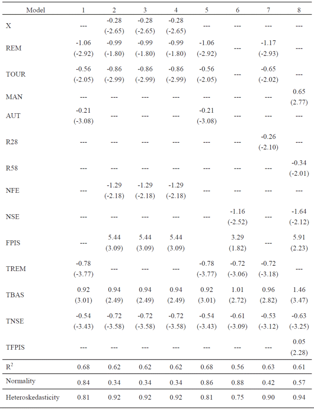
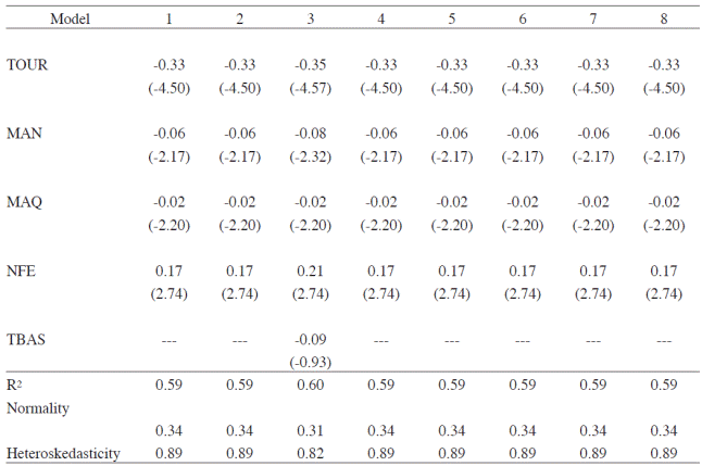
Table 3 Estimation results for the services sector (estimation by OLS)
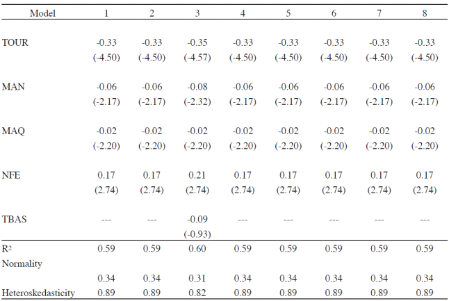
Numbers in parenthesis are t statistics. Figures reported for specification tests are p-values.
Source: Own elaboration.
More specifically, regarding the exposure variables in the case of industrial production, the shares in state GDP of exports (X), remittances (REM) and tourism (TOUR) have negative and statistically significant effects on output drops, as suggested by the literature. In turn, among the specialization variables, when X enters into the model, only the share of transportation equipment in manufacturing production (AUT) is significant and has a negative impact on output drops. In contrast, if the ratio of the basic sector is used as a proxy of international trade (BAS, which is not significant), AUT, R28 and R58 have separated statistically significant and negative effects on output, such as the theory suggests. On the other hand, among the direct effects of the Great Recession, only the growth rate of the basic sector (TBAS) has statistically significant and positive effects on output drops, which suggest that negative external shocks associated to the Great Recession had actually adverse impacts on state production. In addition, there seems to be evidence of a counter-cyclical fiscal policy implemented by the states given that the estimated coefficient of the growth rate of the net state expenditure (TNSE) is negative and significant. On the contrary, the estimation results suggest that the federal fiscal policy has been ineffective and insufficient since the coefficient of the growth rate of federal physical investment in states is statistically significant only in one specification and its sign is positive, implying that the policy was pro-cyclical; this result, however, is not robust. 16
On the other hand, the output drops in the services sector are explained by a small set of variables, as seen in Table 3.17 In general, the estimated models explain nearly 60% of output drops variability. The specific variable that seems to be the most important in the explanation of the tertiary output drops is the ratio of the tourism sector output to state GDP (TOUR), since its estimated coefficient is the greatest one in absolute terms and is statistically significant, which is a quite reasonable result since tourism activities are related to the supply of the most tradable goods and services within this sector. Other variables having negative and significant effects, although their estimated coefficients are small, are the share of manufacturing production in state GDP and the share of “maquila” production in state manufacturing production. To interpret this result, it can be hypothesized that greater exposure in the manufacturing and “maquila” production causes larger output drops that spills over through falls in local employment and income, provoking falls in lower local demand of largely non-tradable goods supplied by the tertiary sector. In turn, among fiscal variables only the net federal expenditure (NFE) has positive and significant effects, a result that is greatly robust, implying that federal fiscal policy has actually been pro-cyclical. Notice that all initial model specifications converge to the same one at the end.
Finally, total output drops are explained by a wider set of variables; the results are reported in Table 4. Consistent with the results yielded by the Moran’s I index, the autoregressive coefficient is negative and statistically significant, suggesting that states with large output drops are neighbors of states with small drops, such as it can be seen in Map 3. The explanatory power of the estimated models varies from 59 to 81% according to the determination coefficients.18 Regarding the explanatory variables, several interesting aspects can be identified. First, most exposure variables have positive and statistically significant coefficients, which is rather odd. A possible explanation may be related to the relatively small size of the ratios IED, TOUR, MAN and BAS as well as to the nature of productive activities, which are largely linked to non-tradable goods and services in many states.19 Second, higher specialization in the production of transportation equipment and, especially, of chemicals and metallic products, machinery and equipment (R25), implies deeper state recessions, as suggested by the literature. Finally, it seems that state government expenditure played no role to mitigate the effects of the Great Recession on the performance of total output, whilst the federal government expenditure contributed to deepen the global recession effects through significant cuts in federal fix investment by state (TFFIS), as indicated by its positive and statistically significant coefficient.
Conclusions
The objective of this paper has been to explain the output drops in the Mexican states provoked by the Great Recession originated in the US. Since the Mexican economy is highly integrated and its business cycles are strongly synchronized to the US economic dynamics, that recession was quickly transmitted to the Mexican economy, with deep and adverse effects on economic activity. Indeed, Mexico experienced a generalized recession across states and sectors, although specific output drops were heterogeneous.
In this paper, quarterly indexes of total, industrial and services production of the Mexican states are analyzed. Spatial (to give account of the recession transmission from one state to another) or cross-sectional regression models have been formulated and estimated to explain differences in the state output drops. However, the specification tests, such as the Moran’s I index and the Lagrange multiplier tests, suggest that spatial autocorrelation is present only in the case of total production.
The explanatory variables were divided in three different sets: measures of exposure to external shocks, specialization patterns and external demand and fiscal shocks. In general, exposure variables were relevant to explain sectorial output drops, but not total declines in production. In particular, industrial output falls can be explained by the share in state GDP of exports, remittances and tourism, while the shares in state GDP of tourism and manufacturing have played an important role in the explanation of recessions in the services sector. The estimated coefficients of most of these variables are negative suggesting that the higher the exposure to external shocks, the larger the state output drops. The specialization variables have also had negative impacts on output implying that the higher the specialization of the state economy in the production of tradable goods (mainly durable goods), the larger the drops in output.
On the other hand, total production shows evidence of negative and significant spatial autocorrelation, which does not support the hypothesis of transmission of the recession from one state to its neighbors. On the contrary, this evidence indicates that states with deep recessions have neighbors with small output drops and vice versa. Regarding the explanatory variables, the results suggest that the specialization in the production of transportation equipment and chemicals and metallic products, machinery and equipment provoked larger drops in total output. In addition, the direct adverse effects of the Great Recession, as measured by the negative growth rate of the basic sector, but not the structural exposure to external shocks, played a significant role in the reduction of the state total production.
Finally, the estimation results suggest that the federal fiscal policies played no role or even amplified the adverse effects of the Great Recession at state level, especially in the case of the total and services production. On the contrary, state government expenditure contributed to mitigate the effects of the recession in the industrial sector only. Overall this evidence reflects a limited or counterproductive performance of the federal and state governments in the stabilization of the effects of the past recession. Nevertheless, looking ahead, it is worth wondering whether this is the best role the governments should play in the context of more open local economies.