1. Introduction

^{Aghion and Howitt (1992)} consider in the context of endogenous growth theory the impact of innovation on economic activity. These authors show that both innovative firms and the amount of work dedicated to innovation tend to increase technological expansion and, as a consequence, the productivity of the economy. Also, under the framework of Schumpeterian endogenous growth, ^{Coe and Helpman (1995)} show that investment in research and development (R&D) drives Total Factor Productivity (TFP). These authors provide empirical evidence of the importance of investment in research, as it should be expected. Also, these authors point out that the expenditure of the trade partners on R&D has a positive effect on TFP in the domestic economy. Moreover, ^{Young's (1998)} work remarks that growth in TFP precedes the expenditure on R&D. Finally, it is worth pointing out that another ^{Aghion and Howitt (1998)} consider that to sustain growth in TFP is necessary to increase spending on R&D.

On the other hand, ^{Zachariadis (2003)} studies U.S. manufacturing and finds that an increase in investment in R&D incentives a patent augment. This raise in the number of patents leads to greater technical progress bringing, in turn, economic growth. In this regard, ^{Aghion et al. (2004)} use panel data to show that the rapid increase in TFP during the eighties in the UK could be linked to trade openness, arrival of foreign firms, market competition, and technological innovation. Also, ^{Ha and Howitt (2007)} show that to maintain growth in TFP is necessary to keep the proportion of gross domestic product (GDP) spent on R&D. These authors develop a hybrid model that considers the capital accumulation neoclassical model of endogenous growth and productivity of the Schumpeterian model finding that between 30% and 70% of the growth in per capita output in the countries of the Organization for Economic Cooperation and Development (OECD) can be attributed to capital, while in the long run all growth in per capita output is caused by technological progress. Finally, ^{Madsen (2007)} studies five developed OECD countries using panel data models and concludes, based on Schumpeterian theory, that an increase in TFP not only is related to the local research strength, but also is affected by the research developed by trade partners.

This paper analyzes the impact of technological innovation on economic growth in Latin America. Specifically, it examines the impact of R&D, the number of patents and high-tech exports on economic growth in twelve countries in the region during the period 1996-2008. To do this, it will be carried out an analysis of dynamic panel data with information from the World Bank in order to find evidence on the relationship of technological innovation and economic growth. With respect to the current research, this study distinguishes in the following regards: 1) it focuses on Latin American economies that account for most of the product in the region (Argentina, Brazil, Chile, Colombia, Costa Rica, Guatemala, Honduras, Mexico, Panama, Paraguay, Peru and Uruguay; 2) it considers a greater availability of data in contrast with previous works; and 3) it develops an analysis of dynamic panel data allowing a greater number of countries, variables and periods.

This paper analyzes the impact of technological innovation on economic growth in Latin America. Specifically, it examines the impact of R&D, the number of patents and high-tech exports on economic growth in twelve countries in the region during the period 1996-2008. To do this, it will be carried out an analysis of dynamic panel data with information from the World Bank in order to find evidence on the relationship of technological innovation and economic growth. With respect to the current research, this study distinguishes in the following regards: 1) it focuses on Latin American economies that account for most of the product in the region (Argentina, Brazil, Chile, Colombia, Costa Rica, Guatemala, Honduras, Mexico, Panama, Paraguay, Peru and Uruguay; 2) it considers a greater availability of data in contrast with previous works; and 3) it develops an analysis of dynamic panel data allowing a greater number of countries, variables and periods.

2. Technological Innovation and Economic Growth

The concern for improving the production of ideas, knowledge and information are the elements that drive technological innovation. To understand this phenomenon it is necessary to explore the environment of technological development and innovation systems, as well as the characteristics of innovation processes. In particular, the innovation system relates the innovative firm with agents such as universities, research centers, regulators, competitors, customers and suppliers. The process of technological innovation brings together several innovation activities of the firm and the relationship with activities, such as, knowledge, technologies, information, human resources, financial and business practices, as remarked by the ^{OECD (2006)}.

The process of technological innovation also includes the generation and knowledge acquisition, investment in R&D, production and marketing, and the links between the aforementioned activities. Diffusion is an important part of the innovation process because it discloses the usefulness of the innovation throughout the economy. The process of technological innovation requires the firm is aware that it is a long and risky process because, often, investment in R&D requires substantial resources in the production and marketing of the novel good and not always the expected return is obtained since another innovation overcoming the former may arise. Needless to say, technological innovation can also provide great benefits for innovative businesses, consumers and society as a whole.

Due to the complexity of the innovation process, some researchers try to focus on a specific variable or activity. For example, ^{Porter (1990)} links innovation with competitiveness, and ^{Cooper (1999)} ties innovation with diffusion; other authors link innovation with training and experience.^{1 Romer (1990)} also shows that the use of a larger number of inputs in the production (new materials and intermediate goods) helps increasing productivity stimulating per capita growth. His innovation model introduces the concept of horizontal innovation (which is the contribution of the number of varieties of intermediate goods in production). To Romer, the per capita income growth is directly related to the productivity of researchers in a country; an outstanding result.

On the other hand, ^{Aghion and Howitt (1992)} propose a model with variables such as: the technological coefficient, the amount of work dedicated to innovation, the production of the intermediate good, and the quantities produced of the final and intermediate goods. They show that the engine of economic growth is the production of technology innovations. This production is linked to the institutional framework, i.e., a market that allows the innovator to be financed and, of course, covered in some way against the risk that the firm may be removed from the market. Now then, by thinking of innovation as a change in the production function, as conceived by Schumpeter, it will be considered a Cobb-Douglas production function with constant returns to scale, namely:

where Y_t is production, K_t is capital,²L_t is labor, A is the technological coefficient, and α and 1 - α, are, respectively, the shares of capital and labor in the product. In order to determine the TFP growth, it will be considered Stiglitz (2004) paper that takes into account the contribution of capital to increase production, which is measured by the increase in the capital percentage multiplied by its market share; and following the same idea, the percentage increase attributable to labor is the increase in labor percentage multiplied by its share. The growth rate in TFP is explained by factors other than labor and capital. Among these factors we may mention the efficient use of resources, technological advance, investment in R&D, patents, and exports products with high technological content. As usual, the TPF is obtaining by taking logarithms in (1), and is given by:

where g_Q is the output growth rate, S_K is the share of capital in the product, g_K is the capital growth rate, S_L is the share of labor in the product, and g_L is the labor growth rate. In what follows, equation (2) will be used to compute the growth rate of TFP.

3. Descriptive Statistics of the Analyzed Variables

The data used in this research was obtained from the World Bank. Gross domestic product (GDP) is the dependent variable, and the rest of the variables will be the independent variables. These are expressed in U.S. dollars in the purchasing power parity in 2000, except variables such as labor and patents that are measured in units. For the econometric analysis, it will be considered a balanced panel data (same number of observations for all countries and all variables) to estimate a dynamic model; the period is restricted to available data. The panel includes twelve Latin American countries in the period 1996-2008. Below are the descriptive statistics of the studied variables.

Table 1 shows the variables used in this research, which are gross domestic product, capital, labor, investment in R&D, patents granted and exports with high technology content, as well as their averages, standard deviations, and minimum and maximum values. The theory predicts that TFP growth varies in proportion to the intensity of spending in R&D. Moreover, in the Schumepeterian endogenous growth theory, the levels of investment in R&D have to be dissimilar between large and small economies.

Table 1 Descriptive Statistics of the Variables under Study. 

Source: Data from World Bank.

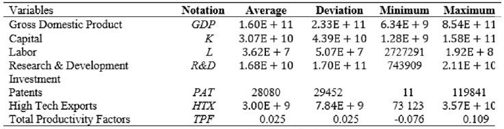
Figure 1 shows that the greatest effort in R&D investment in Latin America is done by Brazil, followed by Chile, Costa Rica, Panama, Argentina and Mexico; however, the differences between Brazil and the other Latin American countries are notorious as Brazil doubles the research intensity of most Latin American countries. Brazil spends 1.1% of its GDP on R&D and is the pointer in Latin America; however, it is still far from global leaders such as Israel and Sweden that spend 4.5% and 4.2% of their GDP, respectively.

Source: Data from World Bank 2008.

Figure 1 Investment in R&D as a proportion of GDP. 

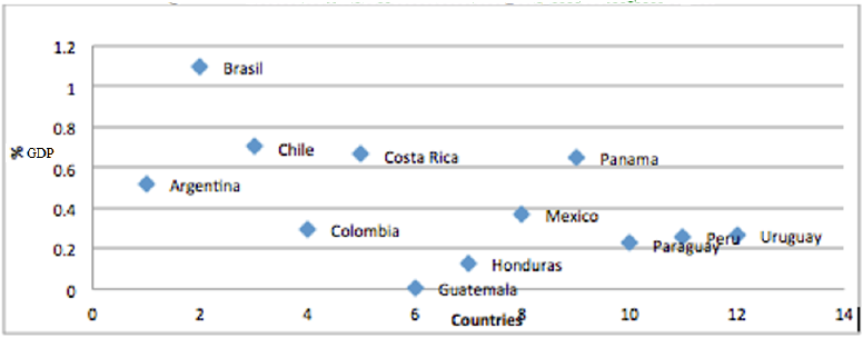
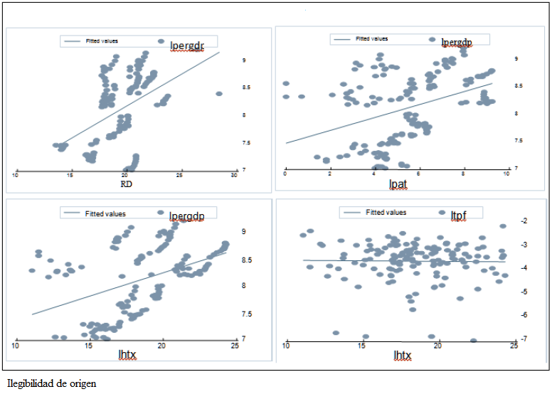
Figure 2 shows that an increase in technological variables has a positive impact on per capita real income. The upper left graph indicates that an increase in investment in R&D raises per capita income. The upper right graph indicates that as the number of patents increases, so does the per capita income. The lower left graph shows that an increase in exports with high technology content leads to an increase in per capita GDP. Finally, the lower right graph indicates that exports of high technological content have little impact on TFP. It is noted that despite the increase in investment in R&D in the region, the effort is poor compared to most developed countries and even in comparison with China. Finally, figure 2 shows the largest impact investment in R&D in the growth rate of per capita GDP compared with the number of patents and high-technology exports.

Source: Data from World Bank.

Table 2 Tech Variables and Per Capita GDP Relationship 

4. Panel Data Analysis

Panel data analysis is a combination of time series and cross-section analysis. The model to be estimated in this investigation is given by:

where y_it is the dependent variable that changes as a function of both i (the number of countries) and t (the number of years), y_(it-1) is the lagged dependent variable, X_it are the exogenous variables y u_it are stochastic perturbations. In this case, the estimates obtained by ordinary least squares (OLS) will be biased. To avoid this limitation, there are some available alternatives by nesting data: fixed effects model (FE) and random Effects (RE), which will be discussed later.

Using panel data has several advantages because it examines a larger number of observations with more and better information, supports a greater number of variables, generates less multicollinearity between data of the explanatory variables, and produces greater efficiency in estimation. Also the use of panel data overcomes the problem of omitted variables that do change over time since they may be removed by taking differences.³

Of course, the panel data analysis has also some disadvantages and limitations as the data become more complex, for instance, heterogeneity and individualities cannot be easily treated. If all the qualities of a country are unobservable, then the errors will be correlated with observations and OLS estimates will be inconsistent. The fixed effects (FE) model involves fewer assumptions about the behavior of residuals. In this case:

It is supposed that ε_it = v_i + u_it That is, the error ε_it can be decomposed into two parts, a fixed constant for each country v_i, and random term u_it that meets the OLS(ε_it = v_it + u_it), which is equivalent to performing a general regression and to give each individual a different origin point (ordinate). The random effects model (RE) has the same specification as the fixed effects except that the terms v_i, rather than being a fixed value for each country that remain constant over time is a random variable with mean value E[v_i] and variance Var(v_i) ≠ 0. The RE model is more efficient but less consistent than the FE. For the estimation of dynamic panel data it is common to use the Generalized Method of Moments (GMM); see, for example, ^{Arellano and Bond (1991)}. They extend the GMM estimation in differences on the basis of regressions in differences to control unobservable effects. They also use previous observations of explanatory variables and lags of the dependent variables as instruments.

The MGM in differences has some limitations as shown by ^{Blundell and Bond (1998)}, particularly when the explanatory variables are persistent over time. The lagged levels of these variables are weak instruments for the difference equation. Moreover, this approach biases the parameters if the lagged variable (in this case the instrument) is very close to being persistent. These authors propose to introduce new moments on the correlation of the lagged variable and the error term. To do this, some conditions are added, namely, the covariance between the lagged dependent variable and the difference of the errors, and the error level must be zero. The GMM system estimator uses a set of difference equations that are instrumented with lags of the level equations. This estimator also relates a set of equations in levels instrumented with lags of difference equations (^{Bond, 2002}).

In the GMM system estimator it is necessary imposed orthogonality conditions to ensure consistent estimates of the parameters even with endogeneity and not observed individual-country effects. This approach will be used here to estimate the parameters from the procedure developed by ^{Arellano and Bover (1995)}, and other improvements provide by ^{Blundell and Bond (1998)}. The estimator thus obtained has advantages over other estimators as FE and others, and does not skew the parameters in small samples or in the presence of endogeneity. In this case, the optimal GMM estimator has the following form:

The above equation is a system consisting of a regression that jointly contains information in levels and differences in terms of moment conditions

These conditions will be applied to the first part of the system. Regression on differences and time conditions, which are written below are applied to the second part i.e., the regression in levels:

The lags of the variables in levels are used as instruments for the regression in differences, and only the most recent differences are used as instruments for the regression in levels. The model generates consistent and efficient estimated coefficients, and also information in differences in terms of

The error component v^*_i proceeds from both models, both levels as differences, which can be defined as:

The matrix of instruments for the model of differences includes information on the explanatory variables and the lag of the dependent variable:

While in the matrix of instruments for the equation in levels only consider explanatory variables without the lagged dependent variable

The matrix of instruments takes the following form and it is included in the GMM estimator:

Finally, the matrix V_N of the covariance and the moment constarins valid for the optimal case is given by:

Additional tests to ensure the smooth running of MGM are suggested by Arellano and Bond's autocorrelation tests of first and second orders and the Sargan test of overidentifying restrictions in panel data by considering the statistic

This test has a χ² distribution where (ν^) is the vector of residuals, Z is the number of imposed conditions, k is the number of parameters included in the vector β, and p is the number of columns of the matrix Z. Sargan test examines the overall validity of the instruments analyzed. Subsequently, the existence of second-order serial correlation of the differentiated error term is reviewed, and the test is performed under the null hypothesis of no second order correlation.

5. Discussion of Empirical Results

The purpose of this section is to develop a panel data model that allows studying two important aspects when working with unobserved heterogeneity: individual-specific effects and time effects. In regard to specific individual effects, these affect each of the selected countries in the sample and are invariant in time. ^{Wooldridge (2012)} identifies these effects with policy issues in each country, such as strength of institutions and access to technology, among others. Temporary effects are those which apply equally to all individual units. These effects may be associated, for example, to macroeconomic shocks and economic crises that can equally affect all countries in a region.

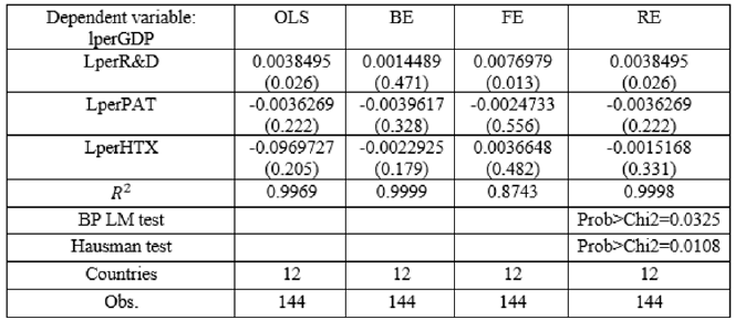
This research focuses on a sample of twelve Latin American countries: Argentina, Brazil, Chile, Colombia, Costa Rica, Guatemala, Honduras, Mexico, Panama, Paraguay, Peru and Uruguay. The analyzed variables are expressed in logarithms of per capita real GDP (lperGDP), per capita investment in R&D (lperR&D), per capita number of granted patents (lperPAT) and per capita high-technology exports (lperHTX). The period under study is 1996-2008, which provides a total of 144 observations. The econometric package Stata.11 will be used to estimate a balanced panel. The main results are shown in Table 2.

Table 2 Estimates Static Panel Data 

Dependent Variable: logarithm of per capita real GDP .

p values in parenthesis.

Source: Data from World Bank .

Table 2 shows the results for four kinds of estimates of static panel data (OLS, "between", and fixed and random effects). The first column indicates that the dependent variable is the logarithm of per capita real GDP. The explanatory variables are the logarithm of per capita investment in R&D, the logarithm of the per capita number of patents, and the logarithm of the per capita high-technology exports. For each estimate, the determination coefficients are computed. Both the Lagrange multiplier and Hausman tests are carried out for each case.

The second column of Table 2 shows the OLS estimate, which provides a significant positive coefficient in investment in R&D, and negative but insignificant coefficients of other technological variables (patents and high-tech exports). It is important to point out that R² is 0.9969.

The third column of Table 2 shows the estimation results "between" (BE), in which none of the variables of interest is significant. There is a positive sign in investment in R&D and an unexpected negative sign in patents and exports with high technological content, and the R² is high, 0.9999.

The fourth column of Table 2 presents the results of the estimation with FE where there is a positive and significant coefficient for investment in R&D, and high-tech exports has the expected positive sign but it is not significant. Patents show an unexpected negative sign but it is not significant. The R² has a value of 0.8743.

The last column of Table 2 shows the estimation results for RE, which indicates a positive and significant coefficient for investment in R&D. Also unexpected negative coefficients for patents and exports are found but they are not significant. Here, the R² is 0.9998. Moreover, Lagrange multiplier provides prob > χ² = 0.3259 which indicates that the RE estimation is preferable to ordinary least squares. Finally, the Hausman test is carried out with prob > χ² = 0.1083 which indicates that the RE estimation is preferable to the FE. Therefore, results indicate that the estimate by RE is the best to explain the impact of innovation processes to economic growth.

Table 3 shows the estimation results of the dynamic panel data regression. As before, the first column indicates that the dependent variable is the logarithm of per capita real gross domestic product. The explanatory variables are the lag of the logarithms of per capita real gross domestic product, per capita investment in R&D, per capita number of patents and the per capita high-technology exports. Tests of serial correlation of the first and second orders, and the Sargan and Hansen tests were carried out.

Table 3 Estimates from Dynamic Panel Data 

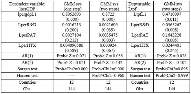
Note: Dependent Variable: logarithm of per capita real GDP.

The second column of Table 3 shows the results of the GMM system estimation in one stage. The coefficients have the expected signs and the lag is significant; while technological variables are not. It is also accepted the serial correlation of first and second order. The Sargan test accepts the null hypothesis, therefore the test supports that the specification of the model and the general validity of the instruments.

The third column of Table 3 shows the results of the GMM system estimation in two stages. All coefficients have the expected signs and are significant. It is accepted the first-order serial correlation, but it is not accepted the one of second order. Sargan test accepts the null hypothesis, therefore it is supported the model specification and the general validity of the instruments. Hansen test is not accepted, indicating the proper use of the instruments as a signal of the proper use of the methodology.

The fifth column of Table 3 explains the TFP of technological variables, finding significant expected positive coefficients, excepting the high-technology exports. Serial first-order autocorrelation is accepted, but the one of second order it is not. Sargan test does not accept the null hypothesis, therefore it is not supported the model specification and the general validity of the instruments. Hansen test is not accepted, indicating the proper use of tools and the suitable use of the methodology. Estimates indicate that the best fit model is GMM system of two-stage, thereby indicating that a 1% increase in investment in R &D leads to an increase of 0.2 % in per capita GDP in the countries of the region, while if patents rise by 1%, then per capita GDP will increase by 0.35%, and, finally, an increase of 1 % of high-tech exports will lead to an increase of approximately 0.1% of per capita GDP. It is also important to note that TFP has greater sensitivity to patents, investment in R&D and high-technology exports.

6. Conclusions

The endogenous growth literature is emphatic in remarking that the innovation generating activities, such as investment in R&D and generation of patents, have important effects on economic growth. Moreover, a greater effort in R&D will drive the increase in TFP and, thereby, promote economic growth. This research showed, first, by analyzing descriptive statistics that investment in R&D, the increase in patents, and the increase in high-technology exports keep a positive relationship with both the per capita real GDP and the increase in TFP for representative Latin American countries. Secondly, the estimates, both static and dynamic, from panel data showed the importance of the technological innovation processes in economic growth and the increase of TFP.

In conclusion, we examined the impact of technological innovation on GDP growth in Latin America. The empirical evidence presented here supports the hypothesis of this paper: there is a positive impact on investment in R&D and other technological variables on economic growth with an increase in TFP for the studied period 1996-2008.

Derived from the present investigation is recommended that Latin American countries should seek the tools and incentives to encourage technological innovation contributing to the increase of TFP, economic growth and, thereby, welfare of the population. Needless to say, it is important to increase the effort in research that can contribute to TFP growth, economic growth and welfare standards of the Latin American population. The raise in investment in R&D in Latin America should be a key objective for policy makers and decision makers in order to foster economic growth and, thus, impulse population welfare.