


Servicios Personalizados
Revista
Articulo
 Inglés (pdf)
 Artículo en XML
 Referencias del artículo
 Enviar artículo por email
Indicadores
-
 Citado por SciELO
 -
 Accesos
Links relacionados
-
 Similares en
SciELO
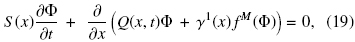
Similares en
SciELO
Compartir

 Permalink
Revista mexicana de ingeniería química
versión impresa ISSN 1665-2738
Rev. Mex. Ing. Quím vol.11 no.3 Ciudad de México dic. 2012
Simulación y control
Operation and design of a liquid fluidized bed classifier for polydisperse suspensions of equal-density solid particles through modeling and simulation
Operación y diseño de un clasificador de lecho fluidizado líquido para suspensiones polidispersas de partículas sólidas de igual densidad por medio de modelado y simulación
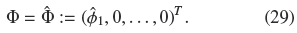
A. García1,2* and G. López3
1 Departamento de Ingeniería Metalúrgica, Facultad de Ingeniería y Ciencias Geológicas, Universidad Católica del Norte, Antofagasta, Chile. * Corresponding author. E-mail: agarcia@ucn.cl 56 55 355645; Fax: 56 55 355664
2 Centro de Investigación Científico Tecnológico para la Minería, CICITEM, Antofagasta, Chile.
3 División El Salvador, Codelco, Chile.
Received 13 of September 2011
Accepted 4 of June 2012
Abstract
For polydisperse suspensions with equal-density solid particles and continuous particle size distribution, design and operation methodologies of a liquid fluidized bedclassifier (LFBC) ere mtroduced, both based on a modified version of the generalized clarifier-thickener (GCT) model presented by Bürger, García, Karlsen, y Towers (2008) Computers and Chemical Engineering 32, 1181-1202. The LFBC is a special case of the GCT characterized by an upwards-directed flow of liquid at the lower end of the unit. Moreover, a versatile way to discretize the particle size variable for the numerical solution of this equation is presented. Numerical examples illustrate the performance of the model and the effectiveness of design and operation methodologies.
Keywords: suspension, fluidization, modeling, simulation, classifier, design, operation.
Resumen
Para suspensiones polidispersas de partículas sólidas de la misma densidad y distribución continua de tamaño, se presentan metodologías de diseño y operación de un clasificador de lecho fluidizado líquido (LFBC), ambos basados en una version modificada del modelo del clarificador-espesador generalizado (GCT) presentado por Bürger, García, Karlsen, y Towers (2008) Computers and Chemical Engineering 32, 1181-1202. El LFBC es un caso especial del GCT que se caracteriza por un fluja de líquido dirigido hacia arriba en el extremo inferior de la unidad. Por otra parte, se presenta una forma versátil de discretizar la variable de tamaño de las partículas para la solución numérica de esta ecuación. Ejemplos numéricos ilustran el funcionamiento del modelo y la eficacia de las metodologías de diseño y operación.
Palabras clave: suspensión, fluidizacion, modelado, simulación, clasificador, diseño, operación.
1 Introduction
Mixtures of disperse solid particles of diverse size and/or density in a fluid, called solid-fluid polydisperse suspensions, are encountered in operations as diverse as mineral processing and food industry, where usually, it is important to group together particles of similar sizes or densities, which is called classification. The classification of particles in solid-liquid systems has been the subject of many theoretical and experimental investigations for several decades.
When a polydisperse suspension is subject to sedimentation, particles of different densities and sizes settle at distinct velocities. Consequently, the final sediment consists of several layers of different composition of particles. This form of segregation is known as differential sedimentation, with faster settling species forming the bottom-most layers, and is commonly used to classify particles in industrial processes. For a system consisting of N different sizes, but equal densities, of particles, N zones of settling suspension are formed, with clear liquid above and a sediment layer at the bottom. The lowest zone, just above the early sediment boundary, contains all particle species at their initial concentration, whereas the region immediately above it is devoid of the largest particles. Each successive zone contains one fewer species than the zone below, with the upper zone containing only the smallest particles.
The author and collaborators (Bürger et al., 2008) present a model for continuous separation and classification of polydisperse suspensions, which extends the model of clarifier-thickener (CT) (Berres et al., 2004; Bürger et al., 2004; Diehl, 2006; Zeidan et al., 2004). The feature is singular sinks describing the continuous discharge of products at several points, whose composition will vary during a transient startup procedure. The well-posedness of the resulting model and the convergence of a numerical scheme for N = 1 are proved by Bürger et al. (2006). They therein formulate a model for a generalized clarifier-thickener (GCT) setup, which may include several sinks, can be operated as a fluidization column, and is allowed to have a varying cross-sectional area. They also define a numerical scheme for its simulation.
Several groups of researchers have conducted experiments with separation devices that are special cases of the GCT setup, and proposed mathematical models for them. Nasr-el-Din et al. (1988; 1990; 1999) study columns for the gravity separation and classification of polydisperse suspensions, that have a feed source at a central depth level and, which are tapped near the top and bottom ends. They also present a mathematical model for the steady-state case only. Experimental results for a similar setup are also presented by Spannenberg et al. (1996). Chen et al. (2002a; 2002b) carry out experiments and develop models of a liquid fluidized-bed classifier for steady state (Chen et al., 2002a) and for the transient case (Chen et al., 2002b). A closely related experimental study is that of Mitsutani et al. (2005).
There are many papers about design and operation for separators and classifiers. On design of thickeners with methods based on Kynch's theory exist the papers by Talmage and Fitch (1955), Hassett (1958; 1968), Moncrieff (1963/64), Wilhelm and Naide (1981), Lev et al. (1986), Waters and Galvin (1991), Yong et al . (1996) and Chancelier et al . (1997), see also the reviews by Concha and Barrientos (1993) and Schubert (1998); based on computational fluid dynamics (CFD) and numerical simulation there are the articles of Kahane et al. (2002), Garrido et al. (2003), Martin (2004) and Burgos and Concha (2005). On design of hydrocyclones with empirical models, there are the works by Castilho and Medronho (2000) and Kraipech et al. (2006); and with CFD there are the articles of Olson and Van Ommen (2004), Slack et al. (2003) and Delgadillo and Rajamani (2005a; 2005b; 2007).
In this paper, we propose a methodology to design a liquid fluidized bed classifier (LFBC) for suspensions with solid particles of equal-density and continuous particle size distribution, and present a methodology of operation of a LFBC. We also modify the model for continuous separation and classification of polydisperse suspensions proposed by Bürger et al. (2008), by considering a hindered-settling factor whose exponent depends on the size particle and a continuous formula for that exponent, among others. Moreover, a versatile way to discretize the particle size variable for the numerical solution of this equation is introduced. We present numerical examples, in part adopting data from the literature.
2 Mathematical model of polydisperse suspension sedimentation
Kinematic models are common approximate descriptions for multiphase flows that are essentially one-dimensional, for example in columns and ducts that are aligned with the driving body force. Usually, in these applications one continuous phase (for solidliquid suspensions, the fluid), and N disperse phases (solid species) are distinguished. We here consider polydisperse suspensions with a finite number N of solid particle species, where particles of species i have mean diameter di and density ρi, and di ‡ dj or ρi ‡ ρi for i ‡ j.
Kinematic models are based on the specification of the velocity of each species relative to that of the fluid as a function of the local concentrations of all species.
For batch settling, this leads to a strongly coupled system of N nonlinear and spatially one-dimensional scalar conservation laws for the vector Φ := (Φ1...,ΦN)T of volume fractions of all species. The extension to a continuously operated clarifier-thickener (CT) unit with a singular feed source leads to a system with an additional transport flux whose velocity is a discontinuous function of the spatial position.
A one-dimensional description is adequate, since for small particles in liquid-solid fluidized beds, velocities and compositions are mostly constant on the perpendicular plane to the direction of gravity force. In addition, the model used herein is supposed to form the basis of design and control calculations, for which low computational cost is desirable. This view is implicitly adapted in many engineering treatments of fluidized beds, see for example (Chen et al., 2002a; Chen et al., 2002b; Greenspan and Ungarish, 1982; Kim and Klima, 2004; Nasr-El-Din et al., 1988; Nasr-El-Din et al., 1990; Nasr-El-Din et al., 1999; Zeidan et al., 2004), and other work cited herein.
2.1 Model equations
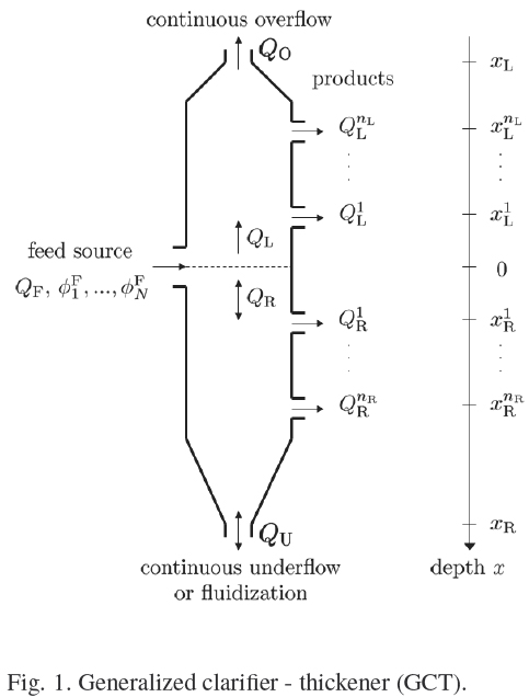
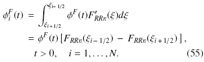
We consider a vessel as shown in Fig. 1. We denote by Φ : = Φ1 + ... + ΦN the total solids concentration. If Vf is the fluid phase velocity, and S (x) is the crosssectional area of the vessel at depth x (x-axis has the origin at the level of feeding and growing downward), then the one-dimensional continuity equations for the N solids phases can be written as
Introducing the volume flow,

we obtain by adding eqs. (1) and (2) the mixture continuity equation ∂Q(x, t)/∂x = 0. Since a constitutive equation will be introduced for the solidfluid relative velocities or slip velocities ui := vi - vf,, i = 1,..., N , we use Eq. (3) and ∂Q(x, t)/∂x = 0 to rewrite Eq. (1) as
We define the parameters δi := di/d1 and  := ρi - ρf for i = 1,...,N , and μ := gd1/(18 μf ), where ρf and μf are the density and the viscosity of the fluid, respectively, and g is the acceleration of gravity, in addition, we specify the phase space of physically relevant concentrations as
where 0 < Φmax  1 is the maximal solids concentration.
Within the Masliyah-Lockett-Bassoon (MLB) model (Lockett and Bassoon, 1979; Masliyah, 1979), ui is specified as
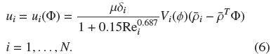
for Rei- < 1000, where  := (1,...,N)T and Vi(Φ) is a hindered settling factor that takes into account the presence of other particles. This function can for example, be chosen as
according to Richardson and Zaki (1954), where ni is a number specified later.
To ensure that the solution assumes values in DΦmax, we herein choose Vi(Φ) as
which continuously goes to zero as F → Φmax and, where Φ < Φq < Φmax is a parameter.
Rei is the particle Reynolds number for species i,
The pair of equations (6) and (9) defines ui implicitly. To avoid this implicit form and to be consistent with previous work, in particular, with the stability analysis of Basson et al. (2009), we approximate Rei by
where β > 0 is a constant parameter that has to be adjusted, and the exponent ni is specified below. Then, we utilize
For spherical particles, the exponent ni depends on the particle Reynolds number at infinite dilution, Re∞,i, and may be given by
according to Garside and Al-Dibouni (1977). Re∞,i, := ρfiv∞, idi/μf is the particle Reynolds number based on the particle settling velocity at infinite dilution, v∞,i, which we calculate as follows (Kunii and Levenspiel, 1991):
Inserting Eq. (11) into Eq. (4) yields the system of conservation laws
where the components of the vector

are the MLB flux functions given by
For the stability analysis of the model for the slip velocity presented here, the reader may refer to work of Basson et al. (2009).
3 The renewed clarifier-thickener model
Bürger et al. (2008) consider a vessel with axisymmetric circular interior cross-sectional area and circular cylindrical outer pipes as shown in Fig. 1. This unit can be operated continuously in two modes, the clarifier-thickener (CT) mode and the fluidization column (FC) mode. In the CT mode, the feed flow is divided into upwards- and downwards-directed bulk flows, and the upper and lower ends of the unit are identified as overflow and underflow levels, respectively, whereas in the FC mode, there is an additional counter-gravity bulk inflow of liquid from x = xR.
We herein subdivide the unit into four different zones: the overflow zone (x < xL), the clarification zone (xL < x < 0), the settling zone (in CT mode) or fluidization zone (in FC mode) (0 < x < xR), and the underflow zone (in CT mode) or water inflow zone (in FC mode) (x > xR). The vessel is continuously fed at depth x = 0, the feed level, with fresh feed suspension, and it has discharge outlets for products at different depths located above and below the feed point.
3.1 Suspension bulk flows
The suspension is fed at the volume rate QF(t) ≥ 0 and, Qo(t) and Qu(t) are the volume bulk flows at overflow and underflow, respectively, where Qu(t) > 0 and Qu(t) ≤ 0 in the CT and FC modes, respectively, and Qo(t) ≤ 0.
Now let us include discharge openings located at  associated with the respective discharge rates
  . We can write the bulk flow as
3.2 Solids feed and sink terms
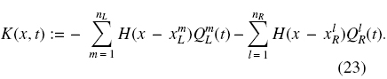
As in Bürger et al. (2008), we assume that for x > xR and x < xL, the cross sectional area shrinks to a very small value, so that these zones actually correspond to transport pipes in which all solids (if any) move with the velocity of the fluid. Consequently, the slip velocities ui,..., uN are "switched off" outside the vessel interior (xL, xR) by the discontinuous function
The next step is to replace Eq. (14) by the system of equations
where Q(x, t) is given by Eq. (17). Next, we consider that at x = 0, the unit is fed at a volume rate QF(t) ≥ 0 with feed suspension that contains solids of species 1 to N at the volume fractions  . We assume
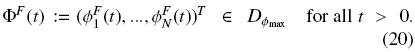
The feed mechanism gives rise to an additional singular source term to Eq. (19), so that we now consider the equation
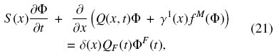
where δ(x) is the Dirac delta function centered at x = 0. Using the Heaviside function we may absorb the right-hand side of Eq. (21) into the flux function. Furthermore, we take into account that the sink terms model the discharge of suspension of unknown concentration. This leads to the equation
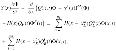
which can be rewritten as
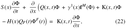
where we define the piecewise constant (with respect to x) function
3.3 Final form of the mathematical model
We assume that the control variables QF(t), Qu(t) and Qo(t) as well as the discharge fluxes controlling the sink terms are constant. Then, in view of Eq. (17), and adding the constant vector -QOΦF into the spatial derivative of the left-hand side of Eq. (22), we can rewrite Eq. (22) as
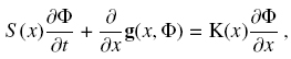
where we define
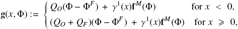
and K(x) is the time-independent version of K(x, t).
Defining the discontinuous parameter
and the vector ϒ(x) := (ϒ1(x), y2(x)), we obtain
This yields the governing equation
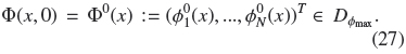
This system is solved together with the initial condition
4 The liquid fluidized bed classifier
4.1 Preliminaries
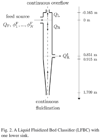
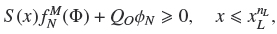
In this section, we determine conditions on the crosssectional area and volume flow rates of a Liquid Fluidized Bed Classifier (LFBC) (see Fig. 2) under which the MLB mathematical model predicts the existence of different compositions inside the unit and of the overflow, underflow and discharge streams, for given volume flow rates QF and Qu, and concentration vector ΦF. We consider suspensions in which the solid species differ in size only (i.e., p1 = p2 = ... = pN =: ps), then Eq. (16) simplifies to the following equation:
4.2 Design of a LFBC
4.2.1. Criterion 1
We choose as first criterion for design of a LFBC that particles of the largest species (species 1) do not leave the column by the underflow, with the purpose of do not block the pipe for the fluidization liquid. Then, in the zone below the lowest sink, the value of the flux of the largest species must be less than or equal to zero, i.e.
from which we obtain
Moreover, we may expect that the largest species is the only present in that zone, so the volume fraction vector has the form
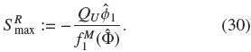
Therefore, for given Qu < 0 and  1such that 0 < 1 Φmax, the maximum cross-sectional area of the column in the fluidization zone is given by
4.2.2. Criterion 2
A second criterion for design of a LFBC is that particles of the smallest species (species N) do not leave the column by the overflow, with the purpose of obtaining a clean liquid. Then, in the zone over the uppermost sink, the value of the flux of the smallest species must be greater than or equal to zero, i.e.
from which we obtain
Moreover, we may suppose that the smallest species is the only present in that zone, so the volume fraction vector has the form

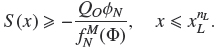
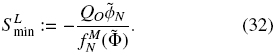
Therefore, for given QO < 0 and  N such that 0 < N Φmax, the minimum cross-sectional area of the column in the clarification zone is given by
4.3 Operation of a LFBC
We denote x+ and x- as the right and left limits of x, respectively. Furthermore, in this section for a general function G(x, t), because t = to is given, we simplify the notation in the following way: G(x+) := G(x+, t0), G(x–) := G(x–, t0).
4.3.1. Volume balance for each species in a node with singular source or sink located at x = 
This volume balance will be useful for studying the bulk flows and concentrations around singular sources and sinks. For species i, Fi(x, t) represents the flux function in x-direction and Fs1 (t) is the singular flux term located at x = , then the volume balance for species i in a control volume with center at x = and thickness 25 is the following
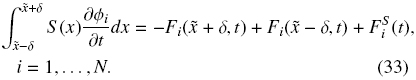
Let δ → 0, then the volume balance for each species at x = results

And as t = t0 is given, we simplify the notation of the above equation as follows:

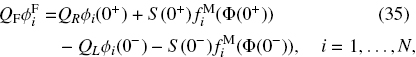
Then, for the volume balance at x = 0 for each species, we apply the Eq. (34) to yield
4.3.2. Condition 1:
Separation of species 1, ... ,m from species m + 1,... ,N in the feed point at x = 0
This condition means that no particles of species 1 to m in x < 0, and no particles of species m + 1 to N in x > 0, or equivalently particles of species 1 to m move downward in x < 0, and particles of species m + 1 to N move upward in x > 0. Then, the following flux relations are valid
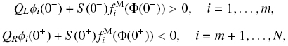
which we replace in Eq. (35) to produce the following relations
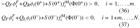
Because of the numeration of solid particles species of same density, relations (36) and (37) can be reduced to the following ones
from which we obtain the relation for our Condition 1

with

and
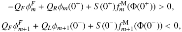
4.3.3. Condition 2: Separation of species m from species 1,... ,m - 1 in the sink point at x = x1R
This condition means that all particles of species m in x > 0 go through the sink at x = x1R. The generalization of this case to others sink points is simple.
First, we require that particles of species m move downward, i.e.
Second, we need that all particles of species m in x > 0 go through the sink, then
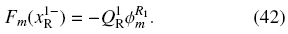
Finally, because the water flow for fluidization, the volume fraction of species m in the sink is less or equal than that above the sink level, i.e.
The Condition 2 of separation of species is obtained combining the relations (41), (42) and (43), in the following one

For the scalar case, the above relation (44) can be derived from the jump conditions given by Bürger et al. (2006).
5 Numerical scheme
5.1 Discretization of the interior of the GCT
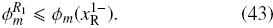
We discretize the spatial domain into cells Ij := [xj-1/2, xj+1/2), j ∈ {0, ±1, ±2,...}, where xk = kΔx for k ∈ {0, ±1/2, ±1, ±3/2,...}. Similarly, the time interval (0, T ) is discretized via tn = nΔt for n ∈ {0,..., N}, where N = [T/Δt] + 1, which results in the time strips In : = [tn, tn +1), n ∈ {0,...,N - 1}. Here Δx > 0 and Δt > 0 denote the spatial and temporal discretization parameters, respectively. We set Δx := L/(J +1) where L is the height of the column and J is a natural number, and Δt is chosen so that the following stability condition (CFL condition) holds:
where p(·) denotes the spectral radius, Jf (ϒ, Φ) the N x N Jacobiano f (ϒ, Φ), and S min = minxx∈(-∞, ∞)S (x).
In the numerical scheme, we approximate max p(Jf (ϒ, Φ)) by

where Smax = maxx∈(-∞, ∞) S (x), and ν1∞ is given by Eq. (13) with d and ps replaced by di and pi, respectively.
We denote by G(x-) the limit of a function G(ξ) for ξ → x, ξ < x, and introduce the difference operators Δ_Vj := Vj -Vj-1 and Δ+ Vj := Vj+1 - Vj
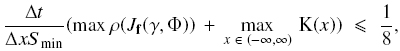
Our scheme is a direct modification of the one described by Kurganov and Tadmor (2000). Let Ujn := (Un1,j, ..., UnN,j)T denote our approximation to Φ(xj, tn). Expressed in terms of the forward Euler solver, we consider the one-parameter family of Runge-Kutta schemes
where ϒj+1/2 := ϒ(x-+1/2), λj := Δt/(Sj Δx) with Sj := S(xj-), Kj := K(xj-), and Uj0 := Φ0(xj-). We employ second-order time differencing (s = 2), for which η1 = 1/2; for third-order time differencing (s = 3), the appropriate values are η1= 3/4 and η2 = 1/3.
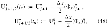
The numerical flux vector h appearing in Eq. (46) is given by
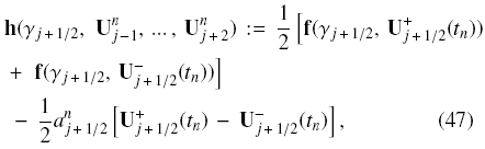
which is expressed in terms of the intermediate values
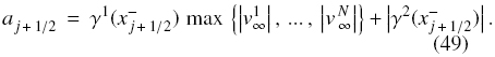
and the local speeds of propagation anj+1/2, which we estimate by
The numerical derivatives are determined by
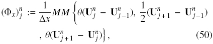
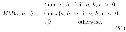
where θ ∈ [1, 2] is a parameter and MM(·, ·, ·, ) is the minmod function:
As stated by Kurganov and Tadmor (2000), in the scalar case (N = 1) the value θ = 2 corresponds to the least dissipative limiter, while θ = 1 ensures the nonoscillatory nature of the approximate solution. The best choice of θ depends on the model considered. For systems, the optimal values of θ vary between 1.1 and 1.5 (Kurganov and Tadmor, 2000). As a compromise, and following previous works (Berres et al., 2004; Qian et al, 2005), we choose θ = 1.3 in all examples.
For the justification of the numerical scheme the reader may refer to work of Bürger et al. (2008).
6 Discretization of a suspension with CPSD
6.1 Reduced size
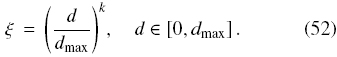
Definition 1. Let d be the particle diameter, dmax be the diameter of the largest particle, and k > 0 a parameter. We define the Reduced Size as
In function of ξ, the Rosin-Rammler particle size distribution is written as
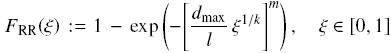
where l is a characteristic size and m is a uniformity coefficient.
Definition 2 (Normalized Rosin-Rammler). Since FRR(1) < 1, we define the Normalized Rosin-Rammler particle size distribution as

6.2 Discretization of a CPSD
We discretize the Reduced Size by defining

for i = 0; ...; N, where N ∈ N and Δξ := 1=N.
Definition 3 (Species in a CPSD). We call "Species i" for i = 1, . . . , N, the solid particles with sizes between ξi+1/2 and ξi+1/2.
Herein, we assign to species i the mean reduced size
If Φn(t) denotes the total solids volume fraction of a feed suspension, the feed volume fraction of the species i is given by
Remark 1. Our definition of the Reduced Size is very useful. For example, when Gates-Gaudin-Schumann CPSD, FGGS(d) := (d=dmax)m, d ∈ [0; dmax], m > 0 is used and if we choose k = 1=m, then ΦiF (t) = ΦF(t)/N. Moreover, if k = 1, then di = dmaxξi, for i = 1; ...; N.
Remark 2. Herein we use the arithmetic mean to determine the mean reduced size of each species, but it is possible to improve the calculation of that, considering the particle size distribution inside each species. Of course, while the number of species be greater, the difference between both means will be less.
7 Numerical examples
7.1 Example 1: Model fit
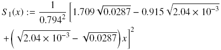
We here adopt experimental data from the work of Chen et al. (2002a) for the steady-state separation of a bidisperse suspension in a liquid fluidized bed classifier. The vessel, Fig. 2, corresponds to equipment "T-2" of Chen et al . (2002a), and is described by its interior cross-sectional area
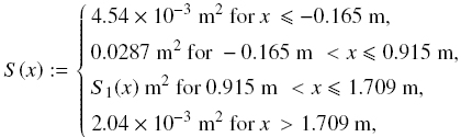
including a conical segment defined by
The solids parameters correspond to glass beads of two sizes. For this suspension, we use Eq. (8) with Φq= 0.63 and Φmax = 0.68, and use Eq. (10) with β = 0.19.
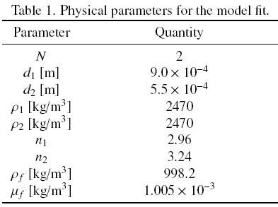
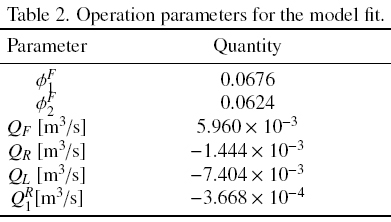
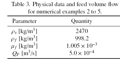
The physical and operation parameters are given in tables 1 and 2, respectively.
In this example we record an approximate L1 error defined with respect to a reference solution, to evaluate the performance of the scheme. We introduce a L1 error, denoted by e1, which is defined by
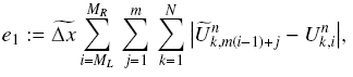
where Ũnk,1 ■ and Unk,1 are the reference solution at x = xi; and the approximate solution at x = xi, respectively, both for species k at t = tn; m is the value of the division between Δx of the approximate solution and that of the reference solution; ML and MR are the indices of the positions between which we calculate the errors of the numerical approximation; and  is the spatial discretization parameter of the reference solution. The reference solution was calculated with the discretization parameters Δx = 3.470 x 10⁻³ m and Δt = 7.352 x 10⁻⁵ s.
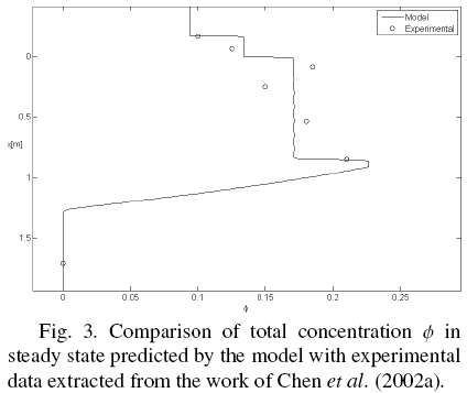
Fig. 3 indicates that the model fits reasonably well the experimental data reported in Fig. 3 by Chen et al. (2002a) that have been obtained by sampling.
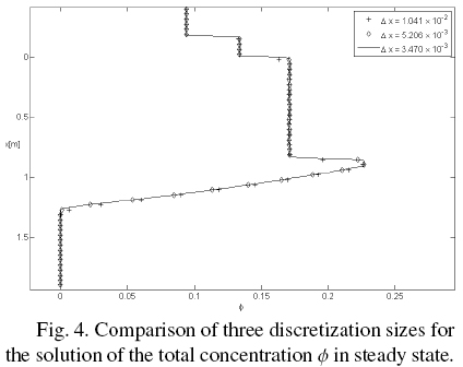
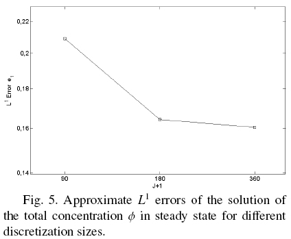
In figs. 4 and 5 we observe that the numerical scheme converges to the reference solution.
Data for next examples
In all next examples, the vessels are similar to that of the model fit (Fig. 2), i.e., it has one only sink located under the feed point. On the other hand, the fluid is water at 20 ºC, the solid is a chalcopyrite concentrate with continuous particle size distribution with Rosin-Rammler parameters dmax = 1.13 x 10⁻³ [m], m = 0.7254 and l = 8.0495, and the reduced size parameter k = 0.5.
The common physical and operational data for the examples are given in Table 3.
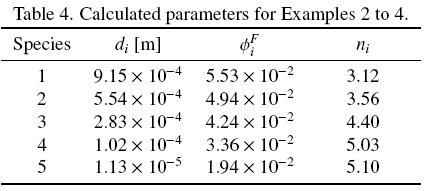
For Examples 2, 3 and 4 the set of particles with continuous size distribution is divided in 5 species. The calculated parameters for they are given in Table 4.
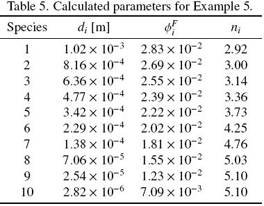
For Example 5 the set of particles with continuous size distribution is divided in 10 species. The calculated parameters for it are given in Table 5.
The operational parameters for numerical examples 2 to 5 are given in Table 6.
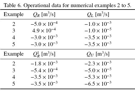
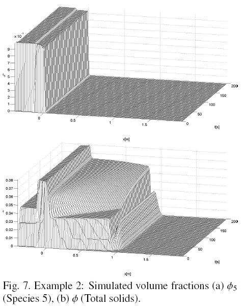
7.2 Example 2: Design of a classifier according to Criterion 1
In this example, the criterion for designing a classifier is that the largest particles must not leave the column by the underflow. The vessel is described by
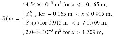
including a conical segment defined by
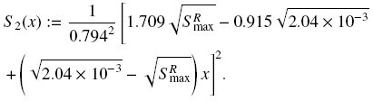
The expected volume fraction of species 1 in the zone below the sink is Φ1 = 0.03. Then, according to Eq. (30), the maximum cross-sectional area in the zone below the sink is SRmax = 1.851 x 10⁻² [m2].
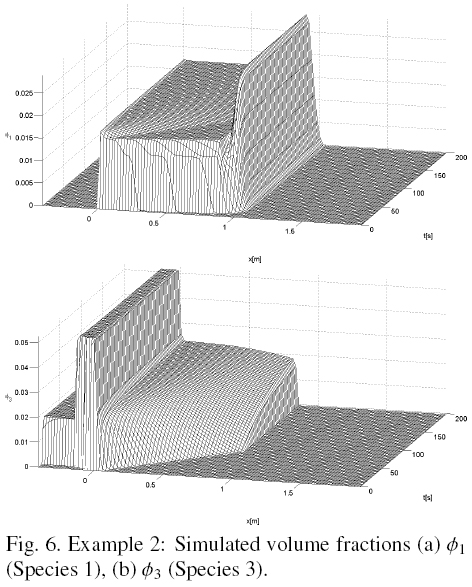
Figs. 6 and 7 show the simulated volume fractions until steady state is reached of species 1 and 3 and, species 5 and total, respectively. Fig. 8 shows the volume fractions of each species and total, versus x in steady state. Fig. 8 shows that the species 1, which is the largest, not output from the underflow and reaches a volume fraction equal to 0.03, which is the expected concentration. Furthermore, it is seen that 1 is the only species present in the area below the sink.
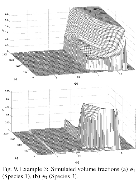
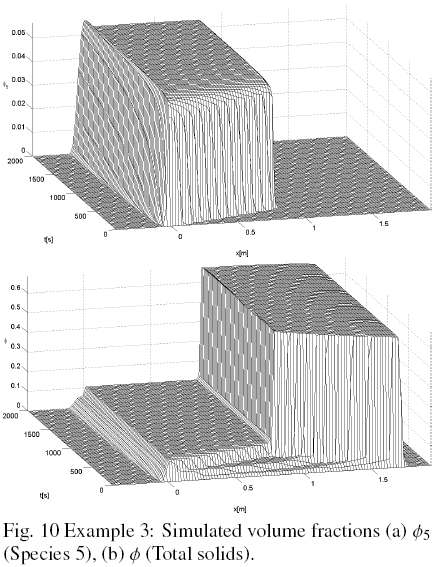
7.3 Example 3: Design of a classifier according to Criterion 2
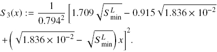
In this example, the criterion for designing a classifier is that the smallest particles must not leave the column by the overflow. The vessel is described by
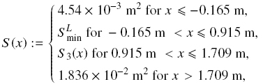
including a conical segment defined by
The expected volume fraction of species N in the zone above the uppermost sink is ΦN = 0.04. Then, according to Eq. (32), the minimum cross-sectional area in that zone is SLmin = 0.1208 [m2].
Figs. 9 and 10 show the simulated volume fractions until steady state is reached of species 1 and 3, and species 5 and total, respectively. Fig. 11 shows the volume fractions of all species and total, versus x in steady state. Fig. 11 shows that the species 5, which is the smallest, not output from the overflow. Furthermore, it is seen that 5 is the only species present in the area above the feeder.
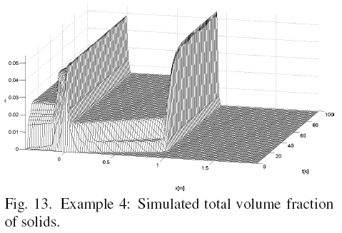
7.4 Example 4: Operation of a classifier enforcing Condition 1
In this example, the condition for operation is that no particles of species 1 to m in x < 0, and no particles of species m + 1 to N in x > 0. The vessel is described by
Figs. 12 and 13 show the simulated volume fractions of species 2 and 3, and total, respectively, until steady state is reached. Fig. 14 shows the volume fractions of each species and total, versus x in steady state. Fig. 14 shows that species 2 and 3 are separated into the feeder. The species 2 that is larger is directed downward, while the species 3 is smaller than species 2 is directed upwards.
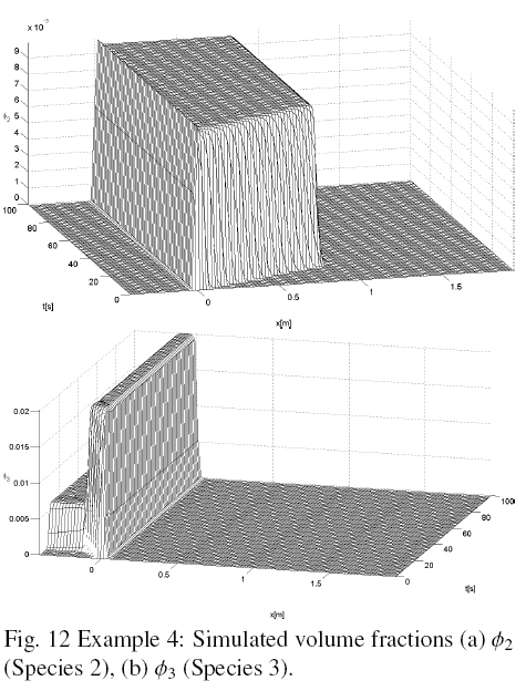
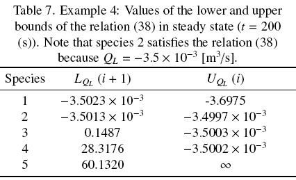
In Table 7, the values of the lower and upper bounds of the relation (38) at time t = 200 (s), when the system is in steady state, are given. Table 7 confirms what is observed in Figs. 12 and 14, in the sense that species 2 and 3 are separated in the feed point, as for the species 2 is satisfied the relation (38).
7.5 Example 5: Operation of a classifier enforcing Condition 2
Here, the condition for operation is that all particles of species m in x > 0 go through the sink at x = x1/R. The vessel is the same of the Example 4.
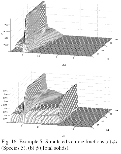
Figs. 15 and 16 show the simulated volume fractions of species 2 and 3, and 5 and total, respectively. Fig. 17 shows the volume fractions of each species and total, versus x near steady state. Fig. 17 shows that in steady state the species 3 does not lower the level of the sink located at x1/R and leaves the unit for it. Species 1 and 2 which are larger, lower-level sink at x1/R.
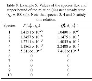
In Table 8, the values of the species flux and upper bound of the relation (44) at time tss = 100 (s), when the system is near steady state, are given. Table 8 shows that not only species 3 and 4 do not cross the level of the sink, as shown in Fig. 17, but so does the species 5, as for these three species satisfies the relation (44).
Conclusions
The contribution of this work is summarized as follows:
• Progress in the model of the generalized clarifier-thickener, presented by Bürger et al. (2008), primarily through the adoption of a hindered settling function for each kind of solid particles.
• Proposition of a method to discretize the variables particle size and volume fraction of species, of a suspension with continuous particle size distribution.
• Presentation of a methodology for designing a liquid fluidized bed classifier (LFBC), in the sense of calculating cross-sectional areas as operational constraints of the equipment, i.e. the non-blocking with solid particles of the pipe that feeds water for fluidization and the collection of clear water by the upper duct.
• Development of a methodology of operation of a LFBC, in the sense of handling the control variables such as volumetric flow at the entrances and exits of the unit, to obtain the desired products.
In the work of Bürger et al. (2008), for all species of particles one hindered settling function V(Φ) are considered, specifically the same exponent in this function, which is calculated as the arithmetic average of the exponents calculated for each species of particles. This assumption we believe is improvable, as in steady state, in the equipment zones of different composition of particles are produced according to their size and density, for example in the case of a suspension of particles of the same density, the lower zone of the equipment is occupied by larger particles, and the upper zone, by smaller particles, so we believe that every species must have its own hindered settling function. Other changes to the model presented by Bürger et al. (2008) are the elimination of the discontinuity in Re; = 0.1 for the formula of the solid-fluid relative velocity ui, the change in the formula for calculating the exponent of the hindered settling function, from the formula of Richardson and Zaki (1954), which is discontinuous, to the formula of Garside and Al-Dibouni (1977), which is continuous, and the relocation of the adjustable parameter in the formula for Rei, so as to increase their range of validity. This work could be useful not only for the design and operation of a LFBC, but also for all equipment whose operation can be modeled with the equations presented here, such as sedimentation of non-flocculated suspensions.
Nomenclature
Acknowledgments
AG acknowledges support by FONDECYT Project 11085069 and Centro de Investigación Científico Tecnológico para la Minería, CICITEM.
References
Basson, D. K., Berres, S. and Bürger, R. (2009). On models of polydisperse sedimentation with particle-size-specific hindered-settling factors. Applied Mathematical Modelling 33, 1815-1835. [ Links ]
Berres, S., Bürger, R., and Karlsen, K.H. (2004). Central schemes and systems of conservation laws with discontinuous coefficients modeling gravity separation of polydisperse suspensions. Journal of Computational and Applied Mathematics 164-165, 53-80. [ Links ]
Burgos, R. and Concha, F. (2005). Further development of software for the design and simulation of industrial thickeners. Chemical Engineering Journal 111, 135-144 [ Links ]
Bürger, R., García, A., Karlsen, K.H. and Towers, J.D. (2006). On an extended clarifier-thickener model with singular source and sink terms. European Journal of Applied Mathematics 17, 257-292. [ Links ]
Bürger, R., García, A., Karlsen, K.H. and Towers, J.D. (2008). A kinematic model of continuous separation and classification of polydisperse suspensions. Computers and Chemical Engineering 32, 1181-1202. [ Links ]
Bürger, R., Karlsen, K.H., Risebro, N.H. and Towers, J.D. (2004). Well-posedness in BVt and convergence of a difference scheme for continuous sedimentation in ideal clarifier-thickener units. Numerische Mathematik 97,2565. [ Links ]
Castilho, L.R. and Medronho, R.A. (2000). A simple procedure for design and performance prediction of Bradley and Rietema hydrocyclones. Minerals Engineering 13, 183191. [ Links ]
Chancelier, J.P., Cohen de Lara, M., Joannis, C. and Pacard, F. (1997). New insights in dynamic modeling of a secondary settler I. Flux theory and steady-states analysis. Water Research 31, 1847-1856. [ Links ]
Chen, A., Grace, J.R., Epstein, N. and Lim, C.J. (2002a). Steady state dispersion of monosize, binary and multi-size particles in a liquid fluidized bed classifier. Chemical Engineering Science 57,991-1002. [ Links ]
Chen, A., Grace, J.R., Epstein, N. and Lim, C.J. (2002b). Unsteady state hydrodynamic model and dynamic behavior of a liquid fluidized-bed classifier. Chemical Engineering Science 57, 1003-1010. [ Links ]
Concha, F. and Barrientos, A. (1993). A critical review of thickener design methods. KONA Powder and Particle Journal 11, 79-104. [ Links ]
Delgadillo, J.A. and Rajamani, R.K. (2005a). A comparative study of three turbulence-closure models for the hydrocyclone problem. International Journal of Mineral Processing 77, 217-230. [ Links ]
Delgadillo, J.A. and Rajamani, R.K. (2005b). Hydrocyclone modeling: large-eddy simulation CFD approach. Minerals and Metallurgical Processing 22, 225-232. [ Links ]
Delgadillo, J.A. and Rajamani, R.K. (2007). Exploration of hydrocyclone designs using computational fluid dynamics. International Journal of Mineral Processing 84, 252-261. [ Links ]
Diehl, S. (2006). Operating charts for continuous sedimentation III: Control of step input. Journal of Engineering Mathematics 54, 225-259. [ Links ]
Garrido, P., Burgos, R., Concha, F. and Bürger, R. (2003). Software for the design and simulation of gravity thickeners. Minerals Engineering 16, 85-92. [ Links ]
Garside, J. and Al-Dibouni, M. R. (1977). Velocity-voidage relationship for fluidization and sedimentation in solid-liquid system. Industrial & Engineering Chemistry Process Design and Development 16, 206-214. [ Links ]
Greenspan, H.P. and Ungarish, M. (1982). On hindered settling of particles of different sizes. International Journal of Multiphase Flow 8, 587-604. [ Links ]
Hassett, N.J. (1958). Design and operation of continuous thickeners. Industrial Chemist 34, 116-120, 169-172, 489-494. [ Links ]
Hassett, N.J. (1968). Thickening in theory and practice. Minerals Science and Engineering 1, 24-40. [ Links ]
Kahane, R., Nguyen, T. and Schwarz, M.P. (2002). CFD modelling of thickeners at Worsley Alumina Pty Ltd. Applied Mathematical Modelling 26, 281-296. [ Links ]
Kim, B.H. and Klima, M.S. (2004). Development and application of a dynamic model for hindered-settling column separations. Minerals Engineering 17,403-410. [ Links ]
Kraipech, W., Chen, W., Dyakowski, T. and Nowakowski, A. (2006). The performance of the empirical models on industrial hydrocyclone design. International Journal of Mineral Processing 80, 100-115. [ Links ]
Kunii, D. and Levenspiel, O. (1991). Fluidization Engineering. 2nd edition. Butterworth Heinemann, Jordan Hill, UK. [ Links ]
Kurganov, A. and Tadmor, E. (2000). New high resolution central schemes for nonlinear conservation laws and convection-diffusion equations. Journal of Computational Physics 160, 241-282. [ Links ]
Kynch, G.J. (1952). A theory of sedimentation. Transactions of the Faraday Society 48, 166176. [ Links ]
Lev, O., Rubin, E. and Sheintuch, M. (1986). Steady state analysis of a continuous clarifier-thickener system. AIChE Journal 32, 1516-1525. [ Links ]
Lockett, M.J. and Bassoon, K.S. (1979). Sedimentation of binary particle mixtures. Powder Technology 24, 1-7. [ Links ]
Martin, A. D. (2004). Optimization of clarifier-thickeners processing stable suspensions for turn-up/turn-down. Water Research 38, 1568-1578. [ Links ]
Masliyah, J.H. (1979). Hindered settling in a multiple-species particle system. Chemical Engineering Science 34, 1166-1168. [ Links ]
Mitsutani, K., Grace, J.R. and Lim, C.J. (2005). Residence time distribution of particles in a continuous liquid-solid classifier. Chemical Engineering Science 60, 2703-2713. [ Links ]
Moncrieff, A.G. (1963/64). Theory of thickener design based on batch sedimentation tests. Transactions of the Institution of Mining and Metallurgy 73, 729-759. [ Links ]
Nasr-El-Din, H., Masliyah, J.H. and Nandakumar, K. (1990). Continuous gravity separation of concentrated bidisperse suspensions in a vertical column. Chemical Engineering Science 45, 849-857. [ Links ]
Nasr-El-Din, H., Masliyah, J.H. and Nandakumar, K. (1999). Continuous separation of suspensions containing light and heavy particle species. Canadian Journal of Chemical Engineering 77, 1003-1012. [ Links ]
Nasr-El-Din, H., Masliyah, J.H., Nandakumar, K. and Law, D.H.-S. (1988). Continuous gravity separation of a bidisperse suspension in a vertical column. Chemical Engineering Science 43, 3225-3234. [ Links ]
Olson, T.J. and Van Ommen, R. (2004). Optimizing hydrocyclone design using advanced CFD model. Minerals Engineering 17, 713-720. [ Links ]
Qian, S., Bürger, R. and Bau, H.H. (2005). Analysis of sedimentation biodetectors. Chemical Engineering Science 60, 2585-2598. [ Links ]
Richardson, J.F. and Zaki, W.N. (1954). Sedimentation and fluidization: Part I. Transactions of the Institution of Chemical Engineers (London) 32, 35-53. [ Links ]
Schubert, H. (1998). Zur Auslegung von Schwerkrafteindickern/On the design of thickeners. Aufbereitungs-technik 39, 593-606. [ Links ]
Slack, M.D., Del Porte, S. and Engelman, M.S. (2003). Designing auto- mated computational fluid dynamics modeling tools for hydrocyclone design. Minerals Engineering 17, 705-711. [ Links ]
Spannenberg, A., Galvin, K., Raven, J. and Scarboro, M. (1996). Continuous differential sedimentation of a binary suspension. Chemical Engineering in Australia 21, 7-11. [ Links ]
Talmage, W.P. and Fitch, E.B. (1955). Determining thickener unit areas. Industrial and Engineering Chemistry 47, 38-41. [ Links ]
Waters, A.G. and Galvin, K.P. (1991). Theory and application of thickener design. Filtration and Separation 28, 110-116. [ Links ]
Wilhelm, J.H. and Naide, Y. (1981). Sizing and operation of continuous thickeners. Minerals Engineering 33, 1710-1718. [ Links ]
Yong, K., Xiaomin, H., Changlie, D. and Qian, L. (1996). Determining thickener underflow concentration and unit area. The Transactions of Nonferrous Metals Society of China 6, 29-35. [ Links ]
Zeidan, A., Rohani, S. and Bassi, A. (2004). Dynamic and steady-state sedimentation of polydisperse suspension and prediction of outlets particle-size distribution. Chemical Engineering Science 59, 2619-2632. [ Links ]

