




 text new page (beta)
 English (pdf)
 Article in xml format
 Article references

 Automatic translation
 Send this article by e-mail
 Cited by SciELO
 Similars in
SciELO

 Permalink

1 Introduction
In recent years, the use and adaptation of orthoses have significantly increased, improving the life quality of many people. Technological advancements allow to develop more durable and adaptive materials, designed to meet the specific needs of users [1]. According to the 2020 INEGI (Instituto Nacional de Estadística y Geografía) census, approximately four million people in Mexico have some mobility disability, although the number of specialists in orthoses and prostheses has been limited, with only around 300 experts reported in previous years [2]. Still, the widespread use of orthoses has been mainly restricted by their high cost, attributed to the materials used in their manufacture and the complexity of control circuits.
Designing orthoses intended to support or correct musculoskeletal deformities or abnormalities, presents several challenges that must be meticulously addressed to ensure both efficacy and comfort for the user. These challenges encompass various aspects, from material selection to customization and biomechanical considerations [3]. One of the primary difficulties in orthotic design is the need for customization. Every patient has unique anatomical features and functional requirements, necessitating individualized orthotic solutions [4]. This demands advanced techniques in measurement and modeling, often involving 3D scanning and printing technologies.
Despite advancements, achieving a perfect fit remains complex, as even minor deviations can lead to discomfort or ineffective support. Biomechanical considerations are integral to effective orthotic design [5]. The device must align and support the body in a manner that promotes natural movement and reduces the risk of further injury [6]. This involves understanding the intricate dynamics of human motion and the forces exerted on different body parts during various activities. Misalignment or improper support can exacerbate existing conditions or create new problems, highlighting the importance of precise biomechanical analysis and the need for feedback-controlled orthoses.
Feedback-controlled orthoses represent an advanced class of assistive devices that incorporate real-time data to adjust their support dynamically [7]. These orthoses utilize sensors and actuators to monitor the user’s movements and physiological parameters, providing adaptive support that responds to the user’s needs and activities.
The integration of biofeedback mechanisms is a critical aspect of these advanced orthoses [8]. Sensors can monitor muscle activity, joint angles, and even stress levels, transmitting this data to a control system that makes real-time adjustments. This capability is particularly beneficial for patients with neurological disorders, where precise control and adaptation are crucial for effective rehabilitation.
Despite their potential, feedback-controlled orthoses face challenges such as the need for sophisticated algorithms, reliable sensors, and user-friendly interfaces. Integration of myography for feedback in various orthosis designs is one of the promising options [9]. To date it is the most reported orthosis control method [10]. Despite its clear advantages, surface myography, the most used for rehabilitation devices, may be sensitive to external noise and present a low signal-to-noise ratio [11]. Additionally, the technique only records potentials, which indirectly indicate muscle fatigue, but does not assess the actual muscle status.
On the other hand, electrical impedance myography (EIM) focuses on the electrical activity and conductivity of muscle tissues and may provide information regarding tissue composition, thus, producing feedback regarding muscle fatigue [12].
EIM consists of applying small-amplitude AC current undetected by the human body and recording the resulting potential. Although electrical impedance has shown promising results in different areas, it is still challenging to apply it to orthosis feedback due to its high sensitivity to limbs´ movement [13].
Another challenge related to EIM is the importance of signal processing to determine muscle fatigue. Fast Fourier Transform (FFT) is a powerful tool for analyzing and designing electrical systems and was successfully applied to other bioimpedance signals [14]. FFT analysis also was proposed to improve feedback for orthosis design [15].
Despite the obvious advantages of EIM, it is still a challenge to apply it in real systems to detect early muscle fatigue.
Since muscle fatigue is a critical phenomenon that can limit mobility and functionality in individuals with neuromuscular disabilities, the development of precise and sensitive technologies such as impedance myography in the context of adaptive orthoses is crucial.
For that reason, the purpose of the present work was to apply FFT analysis to bioimpedance signals obtained in health participants as a proof-of-concept study to establish parameters that may be useful to determine muscle fatigue. Additionally, a simple orthosis design which includes EIM feedback electrodes is presented.
2 Materials and Methods
2.1 Study Desing
A pilot study was conducted to evaluate the effectiveness of an orthosis equipped with bioelectrical impedance electrodes in detecting muscle fatigue in healthy subjects. The study was carried out at the Medical Bioimpedance Laboratory of the University of Guanajuato, Division of Sciences and Engineering. The design included tests at the beginning of the exercise and during muscle fatigue to measure the variation in muscle bioimpedance.
2.2 Participants
Five healthy volunteers (5 men) aged 18 to 26 were recruited. Inclusion criteria were no history of neuromuscular or cardiovascular diseases and good general health. Exclusion criteria included recent injuries to the lower limb and medical conditions that could affect measurements, such as hypertension, diabetes, and respiratory diseases. A preliminary evaluation was conducted before starting the measurement protocol to ensure participants met the inclusion and exclusion criteria.
2.3 Procedure
Volunteers were recruited at the beginning of the study, provided with detailed information about the study, and gave their consent to participate. Initial measurements were taken before the exercise protocol.
Anthropometric Evaluation: Height, weight, and thigh circumference for each participant were measured to calculate body mass index. Additionally, a measurement from the patella of the flexed lower limb to 10 cm proximally to the iliac muscle was taken to determine the starting point for electrode placement on the vastus lateralis muscle.
Procedure: Bioimpedance measurements were acquired using a commercially available BIOPAC MP150. The applied current injection was 400 µA at a frequency of 50 kHz, using superficial Ag/AgCl electrodes, considering the IEC 479-1:1994 standard, which states that the maximum current should not exceed 0.5 mA [16]. A protocol was performed with each participant's non-dominant leg, consisting of multiple 45° extensions or as far as the participant could go without causing injury or pain in or around the knee. Two ankle weights and a resistance band weighing approximately 20 lbs (9.97 kg) were used. The procedure was performed until muscle fatigue was reached, without reaching muscle failure.
Data Collection: data collection involved two measurements: one at the start of the exercise and one at muscle fatigue. The first measurement was taken when the volunteer started the movement. The measurement lasted 15 seconds at a scanning rate of 2500 samples per second, capturing bioimpedance module and phase. After the first measurement, the volunteers continued the exercise protocol until they indicated they could no longer perform extensions, at which point the second measurement, lasting the same duration as the first, was taken. The second measurement was taken during the last 15 seconds of the exercise when muscle fatigue was observed.
Signal processing: the data from each participant was processed separately. First, FFT was performed. The obtained graphs were analyzed and frequencies which presented the most changes before and after the exercise were determined. The Gaussian mask centered at the peak that presented the most change was applied to the FFTs and reverse FFT was performed. The real part of the restored signal was compared before and after exercise conditions.
3 Results and Discussion
For this pilot study, the evaluation was conducted on 5 healthy participants, taking anthropometric measurements illustrated in Table 1. These parameters revealed differences in anthropometric parameters among the participants. Furthermore, based on this information, the design of the orthosis and the configuration of the electrodes were developed, as variations in body dimensions influenced the placement and adjustment of the electrodes, as well as the quality of the data obtained.
Table 1 Results of Anthropometric evaluation for each participant
| # | Height (cm) | Weight (Kg) | Thigh girth (cm) |
| 1 | 166 | 74.5 | 56 |
| 2 | 175 | 90 | 57 |
| 3 | 170 | 90 | 60 |
| 4 | 180 | 75 | 54.2 |
| 5 | 187 | 81.6 | 50.4 |
Figure 1 presents typical graphs of raw bioimpedance data (module and phase). It can be observed that the bioimpedance module followed a wavy pattern: decreasing – muscle contraction, and increasing – relaxation, probably, due to the reduction of muscle length during the contraction.
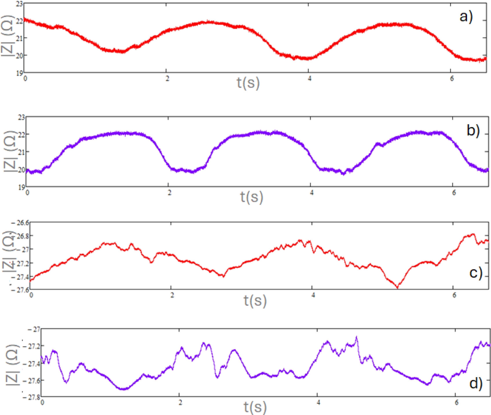
Fig. 1 Representative graphs of raw data bioimpedance module (before (a) and at the end of the exercise (b)), and phase graph (before (c) and at the end of the exercise (d))
Figure 1a shows the raw data for the module, while Figure 1c represents the phase. Both graphs reflect muscle movement at the beginning of the exercise, with measurements taken during the first 15 seconds (the scale of the graphs was reduced to 6 seconds to improve data visualization). In contrast, Figures 1b (module) and 1d (phase) correspond to the last 15 seconds of the exercise, when muscle fatigue is observed. It is obvious that graphs 1b and 1d present more uneven behavior, consistent with involuntary contractions due to muscle fatigue. The raw data graphs were obtained for each participant, allowing the signal to be processed using the Fast Fourier Transform (FFT).
The recorded signals were analyzed in the frequency domain (FFT) to evaluate the characteristics of the signals obtained before and during the presence of fatigue in the vastus lateralis muscle (Figure 2). In Figure 2a, several predominant components in the signal can be observed, where it presents three main peaks indicating the presence of dominant frequencies. The amplitude of the peaks suggests a signal with significant periodic variations. A low noise level is also noted, while still maintaining a clean signal. On the other hand, in graph b, there is an increase in noise level, indicating a greater presence of high-frequency components.
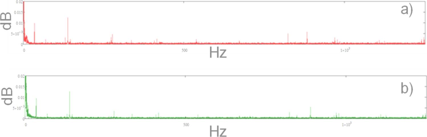
Fig. 2 Typical FFT graph for bioimpedance module signal: a) Before muscle fatigue, b) At the end of the exercise
During muscle fatigue, signal energy became more concentrated in lower frequencies, with a significant reduction observed in higher frequencies. Additionally, the amplitude of the peaks decreased during muscle fatigue, indicating a potential loss of strength or consistency in muscular signals consequently for fatigue. The signal exhibited greater uniformity in the frequency decrease in signal variability.
When analyzing the signals using FFT, the magnitudes in Figure 2 no longer directly represented impedance in ohms (Figure 1) but rather the intensity of the different frequencies present in the signal. For this reason, decibels (dB) were used to express these magnitudes in a standardized way and on a logarithmic scale. Additionally, with the logarithmic scale, the amplitude of low-frequency harmonics could be observed more efficiently across the entire range. Therefore, the x-axis of the graphs was presented on a linear scale.
These alterations in the data could be linked to reduced muscle efficiency and coordination during fatigue, resulting in more uniform signals with diminished energy in higher frequencies.
The distribution of the harmonics in Figure 2 represented the differences between the two measurements taken per participant. Graph a showed the pre-fatigue state, where more pronounced peaks were observed at specific frequencies, indicating the presence of dominant harmonics. In contrast, in graph b (post-fatigue), the harmonics presented lower amplitude, suggesting a weakening of high-frequency harmonics. This reflected a decrease in muscle activity efficiency as fatigue appeared. As the muscle became fatigued, its ability to respond to the injected current was impaired, resulting in a lower amplitude of certain harmonics.
Table 2 presents the data obtained from the FFT analysis of the bioimpedance module before and after the intervention for each participant. The data were organized according to the analyzed frequencies, with changes in amplitude highlighted to identify any increases or decreases in values following muscle fatigue. It can be observed that 5 frequencies were similar between the participants and presented changes in amplitude between studied conditions.
Table 2 Analysis of FFT data obtained from bioimpedance module measurements
| # | Frequency (Hz) | Amplitude (Before), dB | Amplitude (After), | ↑ or ↓ |
| dB | ||||
| 1 | 35 | 0.0074 | 0.0072 | ↓ |
| 277 | 0.0048 | 0.0044 | ↓ | |
| 821 | 0.0048 | 0.0007 | ↓ | |
| 893 | 0.0040 | 0.0005 | ↓ | |
| 978 | 0.0027 | 0.0014 | ↓ | |
| 2 | 35 | 0.0074 | 0.0067 | ↓ |
| 277 | 0.0040 | 0.0044 | ↓ | |
| 822 | 0.0046 | 0.0026 | ↓ | |
| 889 | 0.0091 | 0.0005 | ↓ | |
| 1108 | 0.0018 | 0.0017 | ↑ | |
| 3 | 35 | 0.0060 | 0.0071 | ↑ |
| 277 | 0.0047 | 0.0041 | ↑ | |
| 821 | 0.0043 | 0.0003 | ↓ | |
| 887 | 0.0074 | 0.0001 | ↑ | |
| 969 | 0.0025 | 0.0026 | ↓ | |
| 4 | 35 | 0.0089 | 0.0069 | ↓ |
| 277 | 0.0041 | 0.0045 | ↑ | |
| 822 | 0.0054 | 0.0024 | ↓ | |
| 890 | 0.0081 | 0.0010 | ↓ | |
| 978 | 0.0031 | 0.0021 | ↓ | |
| 5 | 35 | 0.0099 | 0.0095 | ↓ |
| 138 | 0.0125 | 0.0126 | ↓ | |
| 823 | 0.0050 | 0.0026 | ↓ | |
| 883 | 0.0058 | 0.0004 | ↓ | |
| 969 | 0.0031 | 0.0028 | ↓ |
However, only one – 822 Hz, approximately, presented a clear changing pattern (decrease) for all the participants. For that reason, a Gaussian mask centered on this frequency was applied to the signal to isolate the frequency component of interest.
The filtered signal was reconstructed using inverse FFT. The Lissajous graphs were used to represent restored signals before and after the fatigue of the vastus lateralis muscle.
Figure 3 presents a typical Lissajous graph that was used to determine the signal´s real part amplitude. Table 3 presented values from the analysis of the Lissajous graph of the filtered signals from before and after exercise protocol from each participant.
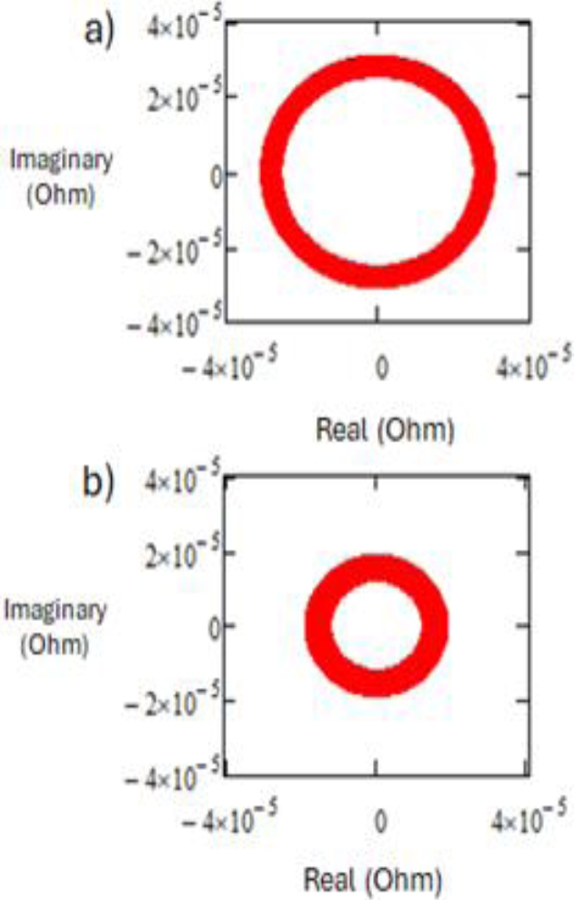
Table 3 Lissajous data analysis measurements
| # | Before | After | ↑ o ↓ |
| (Ohm, 10-5) | (Ohm, 10-5) | ||
| 1 | 2.08 | 2.01 | ↓ |
| 2 | 3.61 | 2.77 | ↓ |
| 3 | 2.65 | 1.91 | ↓ |
| 4 | 3.07 | 1.89 | ↓ |
| 5 | 2.65 | 1.85 | ↓ |
A consistent decrease in the real part of the signal when reaching fatigue was observed. This decrease indicates an improvement in the tissue’s electric conductivity, possibly due to ions´ concentration changes.
The scale of the Lissajous graphs (Figure 3) was associated with high frequencies in the beta (β) range [17], since biological tissue exhibited electrical properties dependent on its composition, cellular structure, and ion and water content. The electrical behavior of the muscle was influenced by charge accumulation at the cellular interfaces, specifically at the cell membranes and the high conductivity of the cytoplasm, along with other components, behaving like a capacitive effect. The β-dispersion occurred when the cell membranes in biological tissues responded to high-frequency electric fields, causing a significant decrease in impedance due to charge accumulation at the interfaces. This meant that the muscle tended to have an electrical response that considerably reduced its resistance, attributed to changes in the cellular structure and ion concentration within the muscle tissue, resulting in reduced impedance values (Table 3).
Similarly to the module graphs, the signals recorded in the frequency domain were analyzed in Figure 4 using the Fast Fourier Transform (FFT) to evaluate the characteristics of the signals obtained in the phase, both before and during the presence of fatigue in the vastus lateralis muscle.
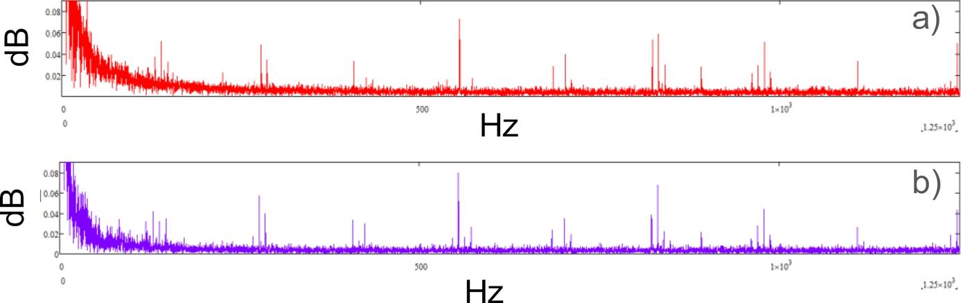
Fig. 4 A representative graph of FFT of EB phase data a) at the beginning, and b) at the end of the exercise
The FFT analysis was also performed for the bioimpedance phase data. Similarly to the module case, changes in amplitude were observed at the beginning and the end of the exercise. However, the detailed analysis (Table 4) did not reveal any specific frequency pattern. The asterisks in Table 4 indicated the frequencies where significant differences were shown between the before and after conditions (increase).
Table 4 Analysis of FFT data obtained from EB phase measurements
| # | Frequency (Hz) | Amplitude (before), Db | Amplitude (after), Db | ↑ O ↓ |
| 1 | 147 | 0.044 | 0.028 | ↓ |
| 277 | 0.056 | 0.055 | ↓ | |
| 554* | 0.075 | 0.079 | ↓ | |
| 821 | 0.05 | 0.002 | ↓ | |
| 830 | 0.054 | 0.022 | ↓ | |
| 2 | 120 | 0.045 | 0.023 | ↓ |
| 424 | 0.05 | 0.038 | ↑ | |
| 554 | 0.05 | 0.033 | ↑ | |
| 831 | 0.083 | 0.068 | ↑ | |
| 1108* | 0.071 | 0.074 | ↑ | |
| 3 | 138* | 0.051 | 0.052 | ↑ |
| 277* | 0.059 | 0.063 | ↑ | |
| 554* | 0.087 | 0.088 | ↑ | |
| 831* | 0.069 | 0.071 | ↑ | |
| 1237 | 0.028 | 0.021 | ↓ | |
| 4 | 138 | 0.052 | 0.031 | ↓ |
| 277* | 0.048 | 0.057 | ↑ | |
| 554* | 0.073 | 0.08 | ↓ | |
| 831 | 0.059 | 0.038 | ↓ | |
| 978 | 0.051 | 0.044 | ↓ | |
| 5 | 146 | 0.052 | 0.045 | ↓ |
| 277 | 0.059 | 0.058 | ↓ | |
| 554 | 0.071 | 0.063 | ↓ | |
| 823 | 0.041 | 0.025 | ↓ | |
| 1116 | 0.031 | 0.026 | ↓ |
The design of a bioimpedance feed-back controlled orthosis intended for persons with reduced mobility was carried out. In Figure 5a, the casing of the orthosis for the lower limb of the thigh is shown, and inside, the skeleton is represented in Figure 5b.
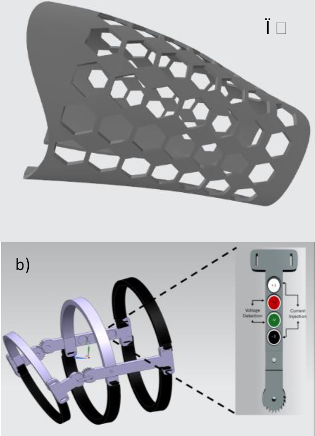
Fig. 5 Orthosis prototype design with electrodes: a) Exterior part of the orthosis, b) Impedance measurement skeleton
The latter one is composed of two sections: one fixed and one movable. In the fixed part, two semicircle rings are placed, one on the thigh and the other on the leg, held by two gears that help the patient perform the movement. The second part has adjustable straps to allow adaptation to any person. Additionally, two support beams are included: one of them was designed for the placement of electrodes, thus optimizing the collection of fatigue samples.
The scale of the Lissajous graphs (Figure 3) was associated with high frequencies in the beta (β) range [17], since biological tissue exhibited electrical properties dependent on its composition, cellular structure, and ion and water content.
The electrical behavior of the muscle was influenced by charge accumulation at the cellular interfaces, specifically at the cell membranes and the high conductivity of the cytoplasm, along with other components, behaving like a capacitive effect. The β-dispersion occurred when the cell membranes in biological tissues responded to high-frequency electric fields, causing a significant decrease in impedance due to charge accumulation at the interfaces. This meant that the muscle tended to have an electrical response that considerably reduced its resistance, attributed to changes in the cellular structure and ion concentration within the muscle tissue, resulting in reduced impedance values (Table 3).
Similarly to the module graphs, the signals recorded in the frequency domain were analyzed in Figure 4 using the Fast Fourier Transform (FFT) to evaluate the characteristics of the signals obtained in the phase, both before and during the presence of fatigue in the vastus lateralis muscle.
The FFT analysis was also performed for the bioimpedance phase data. Similarly to the module case, changes in amplitude were observed at the beginning and the end of the exercise. However, the detailed analysis (Table 4) did not reveal any specific frequency pattern. The asterisks in Table 4 indicated the frequencies where significant differences were shown between the before and after conditions (increase).
The design of a bioimpedance feed-back controlled orthosis intended for persons with reduced mobility was carried out. In Figure 5a, the casing of the orthosis for the lower limb of the thigh is shown, and inside, the skeleton is represented in Figure 5b.
The latter one is composed of two sections: one fixed and one movable. In the fixed part, two semicircle rings are placed, one on the thigh and the other on the leg, held by two gears that help the patient perform the movement. The second part has adjustable straps to allow adaptation to any person. Additionally, two support beams are included: one of them was designed for the placement of electrodes, thus optimizing the collection of fatigue samples.
Correct placement of the electrodes is essential for obtaining optimal and high-quality results. For this reason, it was decided to design an orthosis that contained the electrodes, allowing for precise and reproducible measurements. Additionally, the orthosis follows a standardized procedure that ensures the measurements are consistent and reliable, providing valuable data for evaluation according to the implemented study.
4 Conclusions
The analysis of FFT signals before and after muscle fatigue revealed a clear decrease in energy and signal amplitude at 822 Hz frequency. These findings were consistent with the hypothesis that muscular fatigue affected the efficiency and strength of muscular signals. These results suggested that it is possible to incorporate bioimpedance and its consequent FFT analysis into the design of feedback-controlled orthosis. Future work should focus on expanding the participant group and exploring the underlying mechanisms driving the observed changes in bioimpedance.

