


 nueva página del texto (beta)
 Inglés (pdf)
 Artículo en XML
 Referencias del artículo
 Enviar artículo por email
 Citado por SciELO
  Similares en
SciELO
Similares en
SciELO 
 Permalink
1 Introduction
Computational modeling of natural phenomena and industrial, physical, chemical and biological processes is currently a way to understand them and their interactions (protein interactions, engine combustion, air quality, etcetera). This article describes the configuration and parameterization of physical and computational characteristics required to perform calculations on high performance computers [9, 19, 17] as Mare Nostrum III (BSC-CNS) using the Weather Research and Forecasting model (WRF) in its version 3.5 applied to the Mexico domain [1, 7, 17].
A sensitivity analysis in WRFv3.5 performance was made taking in consideration the effect of the complex topography of Mexico with high spatial resolution [22, 24, 25], being analyzed two nested domains to 3 and 1 km of grid spacing. The simulation of domains was performed using the one-way nesting that is an execution of these two domains that goes from largest to smallest domain [29]. Additional considerations were the analysis of Planetary Boundary Layer (PBL) schemes: YSU (Yonsei University), ACM2 (Asymmetric Convective Models), MYJ (Mellor-Yamada-Janjic) and BouLac (Bougeault-Lacarrére) [6, 12, 14].
According to Krasilnikov et al. [13] “The high diversity of environment in Mexico results from its extent and complex topography. The relief of most of the country is mountainous due to high tectonic activity…” The mountains of Mexico are grouped into diverse systems. The most important systems have been identified as the “Sierra Madre Oriental”, the “Sierra Madre Occidental” and the Transmexican Volcanic Belt. Additionally, it is possible to observe that in the Peninsula of California there are also numerous mountains [13]. Moreover, it is convenient to highlight that Mexico has an abundant highland central plateau, which is enclosed by the “Sierra Madre Oriental” and the “Sierra Madre Occidental”. The plateau has in average 1219 m in elevation in its north region and about 2438 m in the central part of Mexico. The plateau starts in the border with USA and ended in the Isthmus of Tehuantepec. The lowlands of Mexico are Tabasco, Campeche and Yucatán. The highest volcanic peaks of Mexico are Pico de Orizaba or Citaltépetl (5700 m), Popocatépetl (5452 m) and Ixtaccíhuatl (5286 m) [27].
1.1 Problem Definition
The use of NWP (Numerical Weather Prediction) models in Mexico has been extended in the last years, currently being used for example in the National Weather Service (SMN Spanish acronym “Servicio Meteorológico Nacional”) [26], the National Water Commission (CONAGUA, Spanish acronym “Comisión Nacional del Agua) [26] and universities as UNAM or UV among others institutions. The use of NWP is important because the results of these simulations are weather forecasting and support of air pollutants modeling in Chemical Transport Models (CTM) like CMAQ or CHIMERE and may have significant variations in both meteorological and dispersion pollution results if parameterization is not the more adequate.
2 Background and Overview of the WRF Model v3.5
The WRF is a NWP model and atmospheric simulation system designed for both research and operational applications. The model is a multi-agency effort to build a next-generation mesoscale forecast model and data assimilation system to advance the understanding and prediction of mesoscale weather and accelerate the transfer of research advances into operations. The model was developed at the end of the 1990´s with the participation of institutions as the National Center for Atmospheric Research’s (NCAR) Mesoscale and Microscale Meteorology (MMM) Division, National Centers for Environmental Prediction (NCEP) among others [29].
2.1 Model Components, Topographical and Meteorological Considerations
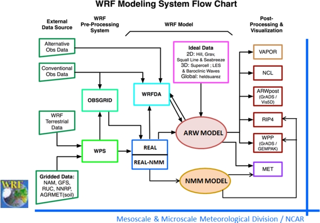
The WRFv3.5 as we see in Figure 1, is structured mainly of three fundamental blocks. The first one is the preprocessing where the files needed are prepared. The preprocessing considers the elevation terrain data and initial meteorological information obtained from global simulations by NCEP or the European Centre for Medium-Range Weather Forecast (ECMWF), among others. The second process is the main step where the dynamic core using the Advanced Research WRF (ARW or NMM) is executed. This process implies the characterization of interfaces and physics packages, considering the necessary schemes according to the site and how the analysis is performed, additionally this process emphasizes the approaches and algorithms running on the solver, physical considerations, initial conditions, boundary conditions and nesting techniques on the grid. Finally the last step is the post-processing in which the analysis of results means validation processes, sensitivity analysis, graphic representation and maps of the interests variables are made [2, 8, 29].
The most used dynamic core is the ARW solver which works with non-hydrostatic Euler equations with the run-time option hydrostatic. At the same time this core uses forecast variables as wind components among others and turbulence regime that considers water vapor, rain, snow, clouds, and chemical tracers’ species.
The studied area needs to be divided into domains with vertical and horizontal coordinates on a grid that considers integration times or time step for calculations based on the initial and boundary conditions configured. Calculation in the interest domains could be done by one-way nesting, two-way nesting or mobile nesting.
The post process analysis is available in the grid selected and can be used from global to high-resolution grids [29].
2.2 Spatial and Temporal Resolutions
The grid complexity of analysis in WRF is given by two factors, the first one is the topography resolution shown in Digital Elevation Models (DEM) taken by default from U.S. Geological Survey (USGS) and the second one the orographic characteristics that define the horizontal resolution, which is the distance or mesh size of the grid in the datasets [16].
These resolutions in both cases should be considered and must be related for the analysis in a specific space, lower grid resolution is less precise and higher resolution is more accurately especially in case of complex topography or in coastal areas [29, 34, 35].
2.3 Configuration Datasets
The initial configuration and conditions consider input data in horizontal and vertical resolution, references of hydrodynamics and disturbance fields and finally the metadata that specifies dates, physical characteristics of the grid and details of the projection. Data preprocessing by the WPS which decodes the information related to orography and land use soil provided by the USGS or initial meteorological data from sources such as NCEP or ECMWF [19] which provide the download datasets in file formats as GRIB, GRIB2, FNL or GFS [5]. These files are processed to generate output files with all variables related [23, 24, 29].
2.4 WRFv3.5 Physics Configurations
Model physics in WRFv3.5 uses schemes ranging from simple, ideals and phase-mixed [2]. Microphysics in this case includes settings for the resolution of water vapor, clouds and precipitation processes. We can see some schemes in Table 1 [29, 31].
Table 1 Microphysics options
| Scheme | Configuration |
|---|---|
| Kessler | 1 |
| WSM6 | 6 |
| Thompson | 8 |
| Morrison 2-Moment | 10 |
Source: Adapted from [29]
2.4.1 PBL Considerations, Configuration and Schemes Available
The parameterization of the PBL is important in the NWP models and should consider the forecast type [21], scale [22], vertical mixing formulation [12, 28], turbulence parameters [17, 24], among others [6, 32, 33], due because occurs in the lower atmospheric layer and interactions with variables and different factors that emphasizing this process in recent decades [1]. The PBL schemes used in this research due to the characteristics in Mexico terrains are shown in table 2 [2, 8, 9].
Table 2 PBL scheme options
| PBL scheme | Configuration |
|---|---|
| YSU scheme | 1 |
| MYJ | 2 |
| ACM2 | 7 |
| BouLac | 8 |
Source: Adapted from [29]
The time step in the WRFv3.5 model use the Runge Kutta 3 (RK3) method in order to maintain physical consistency to numerically solve transport equations, this scheme is limited by the advective number of Courant UΔt/Δx and advection scheme [29], choosing discretization orders for advection terms. This time step [29] is given in seconds and can be estimated by the formula 6 * dx grid size in km chosen for estimation [24, 25].
3 Efficiency and Performance in Parallel Programming
The efficiency and performance in parallel programming usually were assessed by magnitude and performance indicators, using mainly the following metrics: the execution time [10], speed-up and the efficiency [15, 16, 21]. The execution time is the time required for the application for the development of one or more tasks in a program. The performance improvement factor known as speed-up can be estimated by the following expression:
 ,
(1)
,
(1)
where T (n) = execution time in unit steps in time and T (1) = execution time in one-processor
Finally we have to system efficiency for a system with n processors will then:
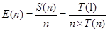 ,
(2)
,
(2)
this efficiency being a comparison of the degree of speed-up obtained from the peak value. Since 1 ≤ S (n) ≤ n, has 1 / n ≤ E (n) ≤ 1.
4 Methodology
4.1 Infrastructure: Mare Nostrum III
The experiments of this research were executed in the supercomputer Mare Nostrum III (MNIII), installed at the BSC. MNIII has a peak performance of 1.1 Petaflop. It has 48896 processors type Intel Sandy Bridge-EP E5-2670 cores at 2.6 GHz. These processors correspond to 3056 compute nodes with 103.5 TB of main memory. MNIII has 1.9 PB of GPFS disk storage. It also has an interconnection network base on InfiniBand and Gigabit Ethernet. MNIII works with Linux operative system Suse distribution 11 SP3 [3].
4.2 Datasets
FNL Datasets of NCEP were downloaded1, we selected grib2 file format prepared operationally every six hours from 2012-05-27 00:00 until 2012-05-28 00:00 with a 1º x 1º grid resolution [19].
4.3 Performance Indicators Experiments
144 experiments were executed to obtain the execution time (t), speedup (Sn) and efficiency (En) considering three hours simulation time with a processors number from 1 to 256, the four PBL schemes (YSU, MYJ, ACM2 and BouLac) [2, 4, 7, 8], two time step and two physics configuration and were executed according to the scheduling in the MNIII supercomputer account [10, 15, 16, 21].
4.4 WRFV3.5 Performance Assessment in Mexico Domains
4.4.1 Description of Mexican Domains
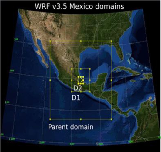
Two nested high resolution domains in Mexico were tested with grids spacing in D1 3 x 3 km2 and D2 1 x 1 km2, parent domain center coordinates were 19.32 LN and -96.54 LW degrees (Figure 2). These domains considered the “Sierra Madre Oriental”, the Trans Mexican Volcanic Belt and the plain coast in the “Gulf of Mexico” in Veracruz, Puebla and Mexico states. The topography presents significant differences in altitude from 32 m.a.s.l. in Veracruz METAR Airport station until 5452 m.a.s.l in Popocatepetl volcano. The topography shows drops in altitude from mountain to flat terrain, with hilly or valleys in the relief [13, 27].
4.4.2 Parameterization in Mexican Domains
The configurations selected for Mexico domains due to topographical and meteorological characteristics, were considered under one-way nesting and for this assessment, executions with differences in configurations of time step values to 18 and 2 seconds considering D1 and D2 with the equation 6 * dx.
50 Eta-levels were automatically configured for the troposphere, microphysics values of 8 and 6 corresponding to 18 and 2 time step were selected, finally PBL models YSU [32, 33], ACM2 [32], MYJ and BouLac [32] for evaluation of PBL in complex terrains conditions such as Mexico topography were assessed [5, 20, 21].
5. Results and Discussions
5.1 Computational Performance
As result of the two settings configured for MPhysics: 8 and 6, the two-time step: 18 and 2 seconds, the number of processors used from one to 128 and the four PBL schemes tested, in Figure 3 we can see that MYJ scheme presented the best execution time, regardless the number of processors and MPhysics used, compared with the other three PBL schemes, which in turn have quite equivalent results.
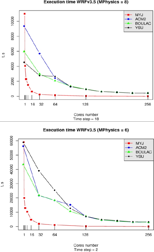
Fig. 3 Execution time results with MPhysics 8 and 6, time steps 18 and 2 and PBL schemes: MYJ, ACM2, BouLac and YSU
With respect to speed up (Figure 4) and efficiency (Figure 5), both results were substantially equivalent.
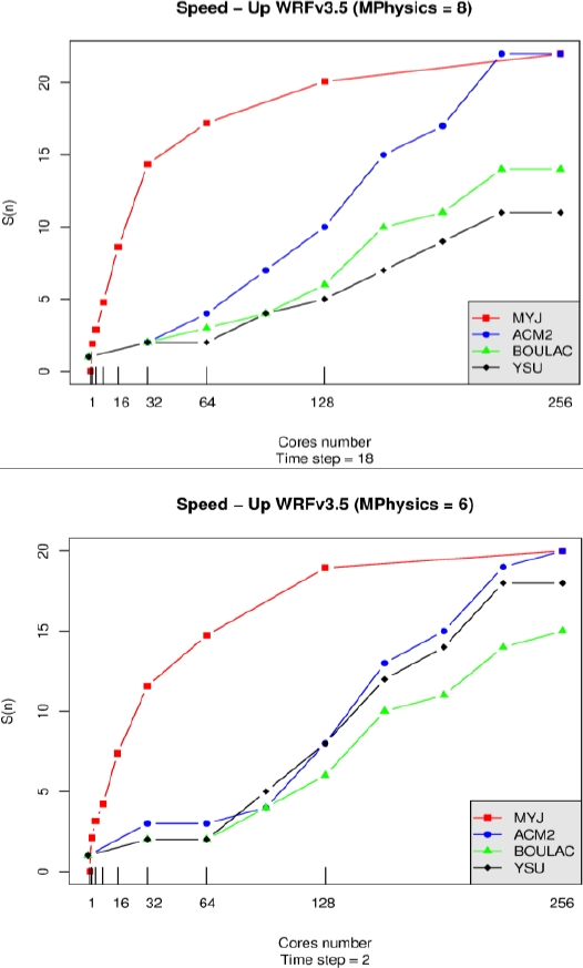
Fig. 4 Speedup results with MPhysics 8 and 6, time steps 18 and 2 and PBL models MYJ, ACM2, BouLac and YSU
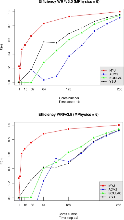
Fig. 5 Efficiency results with MPhysics 8 and 6, time steps 18 and 2 and PBL models MYJ, ACM2, BouLac and YSU
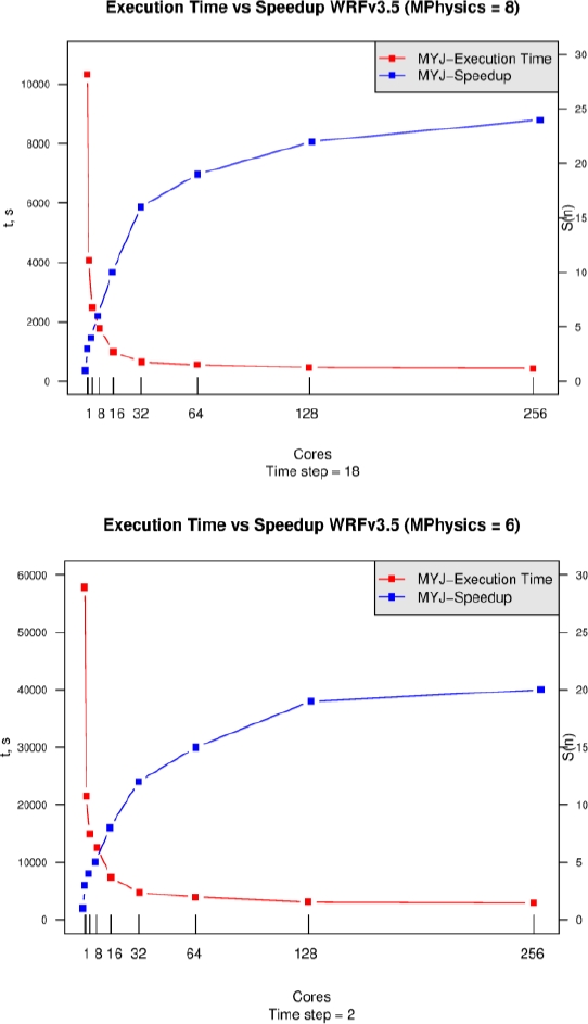
In Figure 6 we can observe a comparative between the execution time and speedup of the MYJ scheme, which was the best parameterization, we can see that intersection in both curves indicates the minimum processors number in both cases are eight processors. It is necessary to consider that execution time observed in MPhysics 8 and time step 18 is smaller than configuration: Mphysics 6 and time step 2.
5.2 Sensitivity Analysis
The sensitivity analysis in nested domain D2 was done using the following meteorological variables: temperature (ºC), wind speed (m s-1) and sea level pressure (hPa) using the MYJ PBL scheme (Mphysics: 8 and two time step: 18 and 2 seconds).
The MB and RMSE were calculated considering meteorological data from METAR station in Veracruz airport, located in 19.09 N and -96.11 W. In Table 3 we can see the results obtained.
Table 3 Sensitivity analysis results for PBL MYJ scheme, Mphysics: 8 and time step: 18 and 2 seconds
| Parameter | Variable | MB | RMSE |
|---|---|---|---|
| Configuration1 (Time step=18) | T(ºC) | 1.4 | 0.1 |
| WS(m s-1) | 0.4 | 0.1 | |
| slp(hPa) | -0.7 | 0.2 | |
| Configuration2 (Time step=2) | T(ºC) | 1.5 | 0.2 |
| WS(m s-1) | 0.5 | 0.1 | |
| slp(hPa) | -0.7 | 0.4 |
We observed the best results with a time step of 18 instead of 2 seconds and insignificant MB differences in T & WS, the MB in sea level pressure is the same value in both cases. On the other hand, the RMSE obtained was considered as a good value.
5.3 Complex Terrain and PBL Accuracy
The PBL MYJ scheme selected was the one with the better results. The complexity in the topography between Veracruz and Mexico states denote the results of the efficiency on computer time, speed-up, and the sensitivity results. Also, the Veracruz METAR Airport station is locate in a coastal area in the Gulf of Mexico demonstrating that a higher spatial resolution is more accurately, especially in the case of complex topography or in coastal areas due mesoscale process, as in these experiments realized [25].
6. Conclusions and Future Work
In this paper we assessing the performance of WRFv3.5 for a domain located between Veracruz, Puebla and Mexico states with complex topography, it has been found that MYJ PBL scheme shows the best performance indicators parameterization with MPhysics set to 8 and a time interval 18 seconds.
So when we are talking about the performance of parallel processing in D2 (1 km) with the MYJ PBL Scheme in WRFv3.5, it can be concluded that the parameterization Mphysics 8 and time step of 18 seconds, it gives us the best indicators related with the execution time and efficiency. Also it was found that the minimum number of processors that could be selected is 16 and over.
The sensitivity analysis performed shows MB and RMSE with a significant improvement in T and WS results between the time step configuration from 18 and 2, the sea level pressure presented good accuracy with insignificant differences. Then these last results should be considered if a good model approximation is required. This means that greater execution time and greater number of processors will be required to achieve these objectives.
Another important conclusion is that these comparisons give us relevant information for operational forecast, key aspect to consider for the managing of computational resources in large domains with high spatial resolution for the mesh (1 km).
As future work, it is necessary to consider the assessment in more days and sites in Mexico with more meteorology METAR stations and the parameterization selected for an accurate model evaluation and an evaluation related with the CMAQ model in the same sites and days assessed.

