


 nueva página del texto (beta)
 Inglés (pdf)
 Artículo en XML
 Referencias del artículo
 Enviar artículo por email
 Citado por SciELO
  Similares en
SciELO
Similares en
SciELO 
 Permalink
INTRODUCTION
Energy is a crucial factor in worldwide development and prosperity. Nowadays, societies are widely dependent on non-renewable energy sources, which are bounded to Climate Change (Bansal et al. 2013). Because of historical events like the Middle East oil crisis in the 1970s, as well as the concern on the resource’s depletion, there is a priority in renewable energies exploitation (Hosseini et al. 2013, Marques et al. 2017). For this reason, alternative energy sources must be developed at a higher growth rate than the global energy demand (Hijazi et al. 2016, Leonard et al. 2020).
In recent years, the generation of biogas from animal manure has acquired attention in the livestock sector. In the case of Mexico, Gutiérrez (2018) estimated that the capacity of biogas production would reach 95.9 Mm3/year in 2030, and 72.5 GWh/year of electricity generation through biogas, representing 7.2 % of the electricity at national scale by only using cattle livestock capacity. The use of these technologies to small-scale farms could not only strengthen clean and efficient energy production, but also bring economic benefits for the farming activities (Zhang and Xu 2020). Moreover, manure-processing technologies could be helpful to close-the-loop in nutrient fluxes while reducing emissions to the environment (Torrellas et al. 2018). The mitigation of emissions could come with a reduction of environmental impacts in general.
The environmental impacts and greenhouse gas balance of biogas production may vary depending on different factors, such as type of biomass, raw material, spatial factor, and system boundaries, between others (Aziz et al. 2019). The anaerobic digestion (AD) technology can operate in both wet and dry conditions. Some studies identified that, through dry AD of byproducts like crop waste, there is an increase in the biogas’ methane concentration in (Martínez et al. 2018, Riya et al. 2018). Dry conditions of AD allow to mitigate water consumption, and it is also suitable for solid content substrates like farm waste, green waste, and the organic part of household waste (Momayez et al. 2019). Zahedi et al. (2018) have studied the performance of thermophilic dry AD, concluding that a bioreactor can operate safely in these conditions. The development of AD in different conditions of moisture could encourage the feasibility at multiple scales.
Within the global trend of developing more sustainable processes, the inclusion of new technologies is a crucial factor to lead the market demands (Mannheim 2016). Hence, to evaluate the potential impacts of biogas production and usage there is a growing interest in the Life Cycle Assessment (LCA) methodology (Aziz et al. 2019). Zhang and Xu (2020) quantified the environmental benefits of biogas power generation systems for large-scale farms. Their LCA-based analysis showed that their proposal offered more environmental benefits and greater economic efficiency compared to an equivalent coal-fired project. Meanwhile, Wang et al. (2018) carried out a comparison between a large-scale biogas scenario and household biogas production in China. They concluded that the large-scale plant had a better performance compared to the household plant from an energetic and environmental perspective. Through LCA, Ramírez-Islas et al. (2020) assessed the environmental effects of energy production from pig manure treatment by AD at medium-scale. They concluded that flaring biogas has a higher environmental burden than energy production. Garfí et al. (2019) evaluated the environmental benefits of low-cost biogas digesters in Colombia, concluding there is a significant reduction in environmental impacts associated with manure handling, fuel, and synthetic fertilizer use. All available literature focused on production rather than the impact of user consumption in an energy grid. Moreover, the production scale plays a vital role in decision-making. Future studies need to expand the boundary conditions to evaluate the sensibility in an energy grid.
To carry out a good quality LCA study, a compilation of a large amount of data is necessary, which involves making assumptions for methodological choices to complete the life cycle inventories. For this reason, the propagation of uncertainty in the potential impacts may lead to inaccurate interpretations and erroneous conclusions (Chen and Corson 2014, Chiu and Lo 2018). Hence, it is essential to consider the uncertainty of the parameters involved in LCA studies to improve the reliability of the results.
Uncertainty plays a key role in each biogas-stage LCA. Incorporating the propagation of uncertainty in LCA results increases the reliability and improves the confidence of decision-making (Groen et al. 2014). In order to provide reliability to LCA results, some authors have chosen statistical methods and simulation (Laurin et al. 2016, Mendoza-Beltrán et al. 2016). Different scenarios were calculated to analyze the influence of input parameters on LCA output results as a sensitivity analysis (Guo and Murphy 2012). The evaluation of biogas systems from a life cycle perspective might enhance the potential of biogas as a sustainable renewable energy resource, mainly in developing countries (Aziz et al. 2019).
No LCA studies focused on Mexican small-scale biogas systems were found; moreover, there is a lack of research studies on specific environmental impacts. Previous studies did not assess the propagation of uncertainty in biogas Mexican inventories. In this paper, we evaluate five proposed scenarios of electricity consumption that use small-scale biogas plants by using LCA. The sensitivity analysis of the scenarios was carried out trough uncertainty assessment using Monte Carlo simulation to corroborate the reliability of results with 95 % confidence. The results could strengthen future studies aimed at technical decision making in this area, as well as encouraging the implementation of biogas technologies in the Mexican energy mix.
MATERIALS AND METHODS
Focus and scope
The main goal of this LCA is to compare five energy consumption scenarios at a small-scale barn that includes an in situ biogas plant for both manure treatment and electricity production. Five scenarios were built considering the contribution of biogas to the energy mix of the barn at different scales. The LCA in this study followed the stages of ISO 14040:2006 (ISO 2006). The above-mentioned scenarios are:
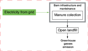
Scenario 1.1. The traditional scenario of dairy manure disposal and electricity consumption of the barn (Fig. 1).
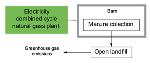
Scenario 1.2. The traditional scenario considering a natural-gas combined cycle power plant (CCPP) as a provider (Fig. 2).
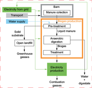
Scenario 2.1. A real case study where 20 % of the manure is treated by AD to produce ~ 40% of the electricity demand by an in situ small-scale biogas power plant (S-BPP). The rest of the consumed energy (~ 60 %) is obtained from the grid (Fig. 3).
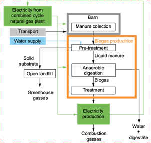
Scenario 2.2. A modification of scenario 2.1, by considering a natural gas CCPP plant instead of the network energy mix (Fig. 4).
Scenario 3. A proposed scenario with 100 % of the manure treated by AD to produce biogas (Fig. 5). All the methane produced with the manure is used for electricity production.
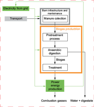
The functional unit for the five proposed scenarios is the energy consumption of the barn throughout one year (104 390 kW/h of consumption). Figures 1-5 show the boundary limits set. The study case used for scenarios 2.1 and 2.2 is a small size biogas plant (~ 22 kW of capacity) located at a dairy farm situated in Chihuahua, México (28º14’ 35” N, 105º 28’14” W). The farm has an average population of 2000 heads of Holstein cattle, and the digester system is located at these coordinates as well. The digester is fully insulated, and it is covered by a bag with a total occupied area of 3169.63 m². The digester is equipped with internal mixers allowing agitation of the slurry. The barn collects ~ 6000 t/yr, and about 20 % of the manure is used for AD (scenarios 2.1 and 2.2). The biodigester produces ~ 200 000 m3 of biogas per year.
Life cycle inventory
Life cycle inventory (LCI) data were collected by three sources: literature, data provided by the producers, and in situ measurements. All the LCI related to infrastructure and indirect emissions were obtained through the Ecoinvent database (Weidema et al. 2013) and the Mexican electricity mix from the grid in scenarios 1.1 and 2.1.
The open landfilling process used in scenarios 1.1, 1.2, 2.1, and 2.2 was built according to the 2006 IPCC Guidelines for national greenhouse gas inventories, Tier 1 for methane emissions from livestock (Paustian et al. 2006). The average year temperature from 1981 to 2014 reported for the specified coordinates was considered (Table S-I in the supplementary material). To calculate potential methane emissions through the manure open landfilling we used equation :
where CH 4 Manure is the methane emission from the manure management in Gg (CH4/yr), EF (T) is the emission factor for the defined livestock population, and N (T) is the number of heads of livestock in a specie T in the country. The calculations considered to build the inventories are shown in table S-II in the supplementary material. We considered 30 % of uncertainty by following the IPCC guidelines recommendations. N2O emissions were also estimated through the IPCC inventory guidelines (Klein et al. 2006). Table S-III shows the calculations for both methane and N2O emissions. Following the recommendations of the IPCC guidelines, a 30 % uncertainty assessment was considered.
For the S-BPP stage scenarios 2.1 and 2.2, all the manure is mixed with water and then separated through a sieve in two phases: a liquid and a solid manure. The first one considers that 20 % of the raw manure in this study is treated by AD. The solid manure is disposed by open landfilling. There are two byproducts obtained from the AD: the digestate, used as composting, and the biogas. Three filters treat the biogas: a NaOH wet scrubber, a silica gel filter, and an activated coal filter. These filters reduce H2S concentration in the biogas mixture. Finally, the biogas produces energy through a turbine of 30 kW of maximum capacity. The study assumes that all biogas generated in the AD process produces electricity. The producers provided this information, and a 30-yr lifetime is assumed for the S-BP. The scenario shown in figure 3 is a common biogas scenario for Mexico where, however, this technology is weakly used. Most of the dairy farms use open landfilling for manure disposal.
Some measurements captured the emissions in the S-BPP for both air and water. Four samples of the water used in the biogas production stage were taken to analyze the initial concentration of pollutants. The samples were digested by the addition of 5 mL of HNO3 on a hot plate at 110 ºC. Another four samples of the effluent were collected as well. They were digested adding an HCl-HNO3 2:1 blend in 1 g of sample in a hot plate at 110 ºC. All samples were collected between the January 18, 2017 and the first week of February of the same year. Inductively Coupled Plasma Optical Emission Spectrometry (ICP-OES) was used to obtain the concentrations of As, Ba, Co, Cr, Mn, Mo, Ni, and Pb in the samples. An ICP-OES iCAP 6500 series model (Thermo Scientific) was used as equipment together with a QCS-27 standard. The ammonium ion was determined with test strips (Macharey-Nagel Nº 91315). For the characterization of turbine air emissions, four samples of combustion gasses from April 26 to May 17, 2017 were collected using Tedlar bags 232 series, with a polypropylene valve. For each sample, 0.5 mL was injected into a gas chromatograph (Autosysten XL Perkin Elmet II) with Porapak Q6FT as a stationary phase and helium as a mobile phase. The carrier gas flow was 20 mL/min, and a heating ramp was 1 ºC/min from 35 to 120 ºC. A thermal conductivity detector was used for the analysis. The samples were introduced through injection.
Other databases were used to complete the LCI. The data collection methods, as well as more detailed information for each unit process, are shown in table I.
TABLE I DATA COLLECTION METHODS FOR EACH UNIT PROCESS OF THE LIFE CYCLE INVENTORY.
| Stage | Data collection method |
| Electricity from grid | The producers covered the electricity requirements for the whole barn. This is considered the energy mix for Mexico from the Ecoinvent database (Weidema et al. 2013). |
| Manure collection | It is collected and transported by a tractor that runs through the pens. The producers obtained the fuel consumption by the tractor and the emissions were calculated using the AP-42 parameters (EPA 1995). The barn infrastructure was considered for the study using the Ecoinvent database (Weidema et al. 2013). |
| Pretreatment process | The tubing was considered as part of the infrastructure. It was obtained from the Ecoinvent database (Weidema et al. 2013). |
| Anaerobic digestion | The producers provided power energy and water consumption by pumping. Biogas production infrastructure was obtained by the producers and complemented with the Ecoinvent database (Weidema et al. 2013). The effluent emission was characterized. It was analyzed by an ICP-OES model iCAP 6500 series (Thermo Scientific) for As, Ba, Co, Cr, Mn, Mo, Ni, and Pb using a QCS-27 standard. Moreover, test strips (Macharey-Nage) were used to quantify NH4 +. Biogas production associated with biomass was calculated from a stoichiometric equilibrium model (Buswell model) with a 70 % yield of the AD system. Values obtained from elementary chromatography analysis were used. |
| Treatment | Caustic soda consumption for biogas purifying was considered using the Ecoinvent database. The tubing was considered as infrastructure. It was obtained from the Ecoinvent database (Weidema et al. 2013). |
| Power energy production | Infrastructure was obtained from the Ecoinvent database (Weidema et al. 2013). Combustion gas emissions were considered as follows: (i) CO2, H2O, and air were obtained by gas chromatography analysis, and (ii) CO, NOx, SO2, particulate matter (PM), CH4, and total organic compounds (TOC) were calculated with the AP-42 parameters (EPA 1995). |
| Water supply | Water consumption was obtained from the producers and the Ecoinvent database (Weidema 2013). |
| Open landfill | Greenhouse gas emissions considered for the study were determined with the 2006 IPCC Guidelines for Greenhouse Gas Inventories (Dong et al. 2006, Klein et al. 2006, Paustian et al. 2006). |
Life cycle impact assessment
Life cycle impact assessment (LCIA) is the characterization of the LCI data into impact categories. This study uses the ReCiPe midpoint impact categories from the Ecoinvent database. The ReCiPe database was developed in collaboration by the Dutch National Institute for Public Health and the Environment, Radboud University Nijmegen, Norwegian University of Science and Technology, and PRé (Weidema et al. 2013). The categories were chosen based on their relevance in other studies, as well as their relation to the main outputs of the LCI. The chosen categories were climate change in kg CO2 equivalent (eq) (CC), human toxicity in kg 1,4-DB eq (HT), terrestrial acidification in kg SO2 eq (TA), water depletion in m3 (WD), and fossil depletion in kg oil eq (FD). The LCIA stage was carried out through the SimaPro 8.4 Ph.D. academic version.
Life cycle interpretation: Sensitivity and uncertainty analysis
LCA results are often subject to uncertainty, which may lead to erroneous conclusions. Hence, uncertainty in LCA is a crucial factor to a better application and congruence of the scope (Pfister and Scherer 2015), thus it is important to consider the uncertainty of all the parameters involved in each case study (Chiu and Lo 2018). The sensitivity analysis was carried out by comparing the five scenarios (Table II). In addition to the sensitivity analysis, an uncertainty analysis for the model output was performed according to variability inventory data. Uncertainty propagation is currently performed in LCA literature by the Monte Carlo sampling method. Caputo et al. (2014) and Dong et al. (2006) recommend the stochastic simulation as a means of addressing data uncertainty. According to Chen and Corson (2014), Monte Carlo simulation is an efficient probabilistic method to estimate the effects of uncertainty on the potential environmental impacts of dairy farms. The Monte Carlo simulation made in Simapro 8.4 software was run with 30 000 iterations at the 95 % confidence level to estimate uncertainties in the assessment of the biogas energy production system from a dairy farm. Lognormal distributed input parameters were considered in this study.
TABLE II CONTRIBUTION OF THE FIVE MAIN SCENARIOS TO THE LIFE CYCLE INVENTORY.
| Unit process | Unit | Scenario 1.1 | Scenario 1.2 | Scenario 2.1 | Scenario 2.2 | Scenario 3 |
| Electricity from grid | kWh | 104 390.00 | - | 61 352.14 | - | - |
| Electricity from combined cycle power plant | kWh | - | 104 390.00 | - | 61 352.14 | - |
| Biogas power production | kWh | - | - | 43 037.86 | 43 037.86 | 104 390.00 |
| Open landfilling | % manure | 100 | 100 | 80 | 80 | - |
RESULTS AND DISCUSSIONS
This chapter is divided into two main sections. In the first section, we discuss the results obtained by the life cycle impact assessment, and compare the scenarios per each impact category used. Table II shows the electricity contribution of the five main scenarios. Scenarios 1.1 and 1.2 considered that the energy network it is considered that andthe CCPP, respectively, satisfy the energy demand. In scenarios 2.1 and 2.2 the energy provided by the S-BPP is equivalent to the energy obtained by 20 % of the manure collected for AD; it is equivalent to ~ 40 % of the energy demand. Scenario 3 considers all the manure collected for AD treatment so that all energy generated is used to cover the energy demand. It is assumed that all energy generated with 100 % of the manure for biogas production supplies all the energy demand. The detailed information of the LCI for each unit process is provided in table S-IV in the supplementary material.
Table III shows the potential impacts per category for each scenario, which are discussed in the following paragraphs. Figure 6 compares scenario 1.1 with the rest of scenarios, establishing equivalences between them. Regarding the climate change category, scenarios 1.1 and 1.2 have the highest impact. It is observed that when a CCPP is considered instead of the energy network, emissions are reduced by up to 113 153.70 kg CO2 eq (23 % of reduction). It is important to consider that scenario 1.2 is a proposed scenario based on the future projection of Mexico, in which the energy sector looks for the implementation of combined cycle systems power plants. Furthermore, scenario 1.2 assumes that the power plant is disconnected from the national network. On the other hand, scenario 2.1 shows a decrease of 269 416.88 kg CO2 eq compared to scenario 1.1, while scenario 2.2 shows a reduction of 222 765.92 kg CO2 eq compared to scenario 1.2, which represents an emissions reduction of up to 50 % in the climate change category.
TABLE III POTENTIAL IMPACTS OBTAINED FOR EACH SCENARIO PROPOSED.
| Impact category | Units | Scenario 1.1 | Scenario 1.2 | Scenario 2.1 | Scenario 2.2 | Scenario 3 |
| Climate change | kg CO2 eq | 4.97E + 05 | 3.84E + 05 | 2.28E + 05 | 1.62E + 05 | 1.34E + 05 |
| Human toxicity | kg 1,4-DB eq | 3.05E + 14 | 1.48E + 06 | 1.79E + 14 | 1.30E + 06 | 2.22E + 05 |
| Terrestrial acidification | kg SO2 eq | 668.37 | 450.77 | 632.39 | 504.50 | 125.14 |
| Water depletion | m3 | 9561.90 | 2.33 | 5625.59 | 7.23 | 2.97 |
| Fossil depletion | kg oil eq | 34 925.08 | 22 316.08 | 32 832.53 | 25 421.97 | 5972.68 |
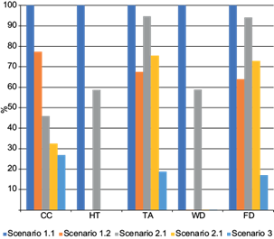
Moreover, the use of energy from the network (scenario 2.1) contributes ~25 % more compared to scenario 2.2 (-66 502.75 kg CO2 eq). Scenario 3 is a proposed scenario where S-BPP completely satisfies the energy demand. An emissions decrease of 94 131.69 kg CO2 eq can be observed in scenario 3 compares to scenario 2.1 (~ 40 % less) and a decrease of 27 628.94 kg CO2 eq (~ 20 %) in scenario 3 compared to scenario 2.2.
Regarding the climate change category, the biogas-related scenarios are beneficial to the mitigation of CO2 equivalent emissions. A reduction of 3.64E + 05 kg CO2 eq was estimated in scenario 1.1 compared to scenario 3 (73 %). Moreover, a reduction of 6.65E + 04 kg CO2 eq (13 %) can be seen in scenarios 2.1 and 2.2, in which the energy grid source changes from a national mix to the CCPP. An emissions reduction of 2.69E + 05 kg CO2 eq was observed in scenario 2.1 compared to scenario 1.1 (~ 55 %). Likewise, there is an emissions reduction of 2.23E + 05 kg CO2 eq in scenario 1.2 compared to scenario 2.2. Scenario 3 considers that all the energy demand is satisfied by the S-BPP, since the total amount of produced manure in the barn is used as substrate. This proposed scenario had the lowest impact, with a total emission of 1.34E + 05 kg CO2 eq.
As for the human toxicity category, scenarios 1.1 and 2.1 show the highest impacts with 3.0534E + 14 kg 1,4-DB eq. On the other hand, scenarios 1.2 and 2.2 had no substantial impact. This pattern is repeated in the water depletion category. In both categories, the scenarios with the energy mix are higher compared to those in which operation units include biogas power and the CCPP. As can be seen in figure 6, the difference between scenarios 2.1 and 2.2 is ~ 99 % (1.79E + 14 kg 1,4-DB eq), and the difference between scenarios 1.1 and 1.2 is ~100 % (3.05E + 14 kg 1,4-DB eq).
In the case of water depletion, the impact of scenario 3 is 9.56E + 03 m3 lower compared to scenario 1.1 and 5.62E + 03 m3 lower than scenario 2.1. Combined cycle power plants use water as heat transporter, which is efficiently recirculated in the system; on the other hand, other traditional thermal power plants emit higher amounts of water. This is observed in the WD impact category, where the amount of water depleted in scenario 3 is 6.44E-01 m3 higher than in scenario 1.2 and 4.26 m3 higher than in scenario 2.2. These results are not concluding by considering a 95 % of confidence, which is further discussed in subsequent paragraphs.
In the category of terrestrial acidification, a lower impact of 2.18E + 02 kg SO2 eq (31 %) is shown in scenario 1.2 compared to scenario 1.1. However, scenario 2.1 has a higher impact compared to scenario 1.2 with a difference of 1.82E + 02 kg SO2 eq (40 %). Furthermore, this behavior shows the contribution of the energy mix in the national network. Scenario 3 shows the lowest impact in this category. Category of fossil fuel has a similar behavior in the impact scores. Fossil fuel consumption is evident in scenarios 1.1 and 2.1, where they provide most of the energy mix in Mexico. The partial consumption of biogas energy shows a lower impact of about 40 %. Likewise, biogas usage from dry bio digestion (scenario 3) has a decrease in this impact by up to 17 %. The contribution in both terrestrial acidification and fossil fuels for scenario 2.2 is higher than scenario 1.2 by ~ 10 %. The main reason is the increase in infrastructure demand for the S-BPP. This pattern is not seen in scenarios 1.1 and 2.1 due to the robust infrastructure in the national grid comparing to the S-BPP. It is essential to consider that 30 years of useful life for the S-BPP are assumed.
Scenario 3 shows the lowest values in all assessed categories. According to Ardolino and Arena (2019) and Ramírez-Islas et al. (2020), the use of biogas shows a better environmental performance if it is equal to the excess of the quantity necessary to satisfy the internal electricity consumption of the system due to savings from electricity self-consumption. This objective is accomplished in scenario 3, and it is corroborated in the LCA results obtained in this study.
The functional unit used in this study is based on the electricity consumption of the barn. This study was looking for a realistic approach to the integration of biogas electricity in agriculture activities. Most of the studies use energy production, biogas production, or even substrate production for their functional unit (Esteves et al. 2019). No studies were found which used energy consumption in these categories to compare. Moreover, most recent biogas studies are focused on the integration of newer technologies, like photosynthetic technologies or even hydrogen production (Wulf et al. 2018, Ferreira et al. 2019).
Uncertainty assessment
Figure 7 shows the uncertainty propagation obtained in the climate change category for each scenario. It is observed that the uncertainty propagation in scenarios 1.1 and 2.1 is too high to be compared with the other scenarios. Besides, figure 7 shows an image enlargement of scenarios 1.2, 2.2, and 3. A reduction of the uncertainty propagation can be observed, compared to scenarios 1.1 and 1.2; this is repeated in scenarios 2.1 and 2.2. Such behavior shows that the usage of the Ecoinvent database for the Mexican energy grid has an important contribution to the uncertainty propagation, which will be explained bellow. On the other hand, scenarios 1.2, 2.2, and 3 have a similar uncertainty propagation. According to the uncertainty propagation, there is a 95 % of confidence that scenario 2.2 is lower than scenario 1.2.
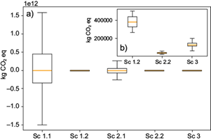
Fig. 7 Uncertainty propagation (standard deviation) of the life cycle assessment for the climate change category.
Figure 8 shows uncertainty propagation for the human toxicity category. As can be seen, it is possible to conclude that scenario 1.1 has a higher impact than scenario 2.1. A high uncertainty propagation is observed in both scenarios, which are out of the 25 % of confidence compared to scenarios 1.2, 2.2 and 3. The reason for this high value is the contribution of the energy mix in the Mexican scenario. As mentioned before, this Mexican energy mix is based on a global energy prospective. The use of thermal power plants powered by fossil fuels such as coal not only highly contribute to climate change, but it also increases human toxicity due to the emission of pollutants such as nitrogen oxides and sulfur oxides. Figure 8 shows an enlargement of scenarios 1.2, 2.2, and 3. The categories show a tendency to higher values in the uncertainty propagation. However, the propagation uncertainty cannot be compared with 95 % of confidence for this impact category.
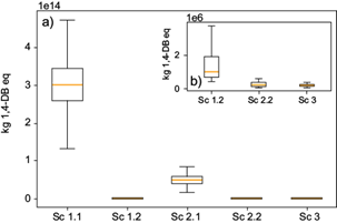
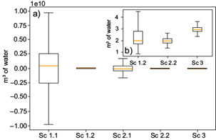
Figure 9 shows the uncertainty propagation for each scenario in the category of terrestrial acidification. As it is observed in the climate change category, the uncertainty propagation makes impossible to compare scenarios 1.1 and 2.1 with other categories. A decrease of 5.37E + 01 kg SO2 eq (12 %) is observed when comparing emissions from scenario 1.2 with scenarios 2.2 and 3; however, this reduction could not be concluded with 95 % confidence. Figure 10 shows the uncertainty propagation for each scenario in the category of water depletion. Even though there is an increase in scenario 3 compared to scenarios 1.2 and 2.2, considering the uncertainty propagation there are no concluding results with a 95 % confidence.
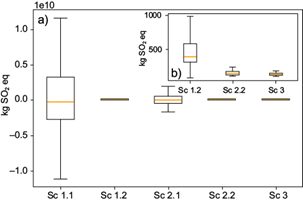
Fig. 9 Uncertainty propagation (standard deviation) propagation for the terrestrial acidification category.
The fossil depletion uncertainty propagation for each scenario is shown in figure 11. As it can be seen, the uncertainty propagation for scenarios 1.1 and 2.1 is too high to be compared with the other categories. On the other hand, it can be observed that scenarios 2.2 and 3 are lower enough to reduce the impact comparing to scenario 1.2 with a 95 % confidence.
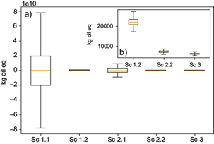
Uncertainty propagation in scenarios 1.1 and 2.1 in all selected categories (except for human toxicity in figure 8) is too high to be compared with the other scenarios (Figs. 7, 9, 10, and 11). This is due to the high uncertainty in the LCI of the Mexican energy grid in the Ecoinvent database, which compiles the LCIs of the energy mix of most countries in the world. However, about half of the countries’ energy mixes were calculated based on the global projections in the energy market instead of local scenarios and/or projections in the energy grid (Vandepaer et al. 2019). Moreover, no other LCI related to the Mexican energy mix was found. Likewise, there are few studies related to the Mexican electricity market. Some studies focus on energy consumption and its CO2 emissions from household energy consumption (Rosas-Flores et al. 2010, 2011). Even though there is a need for accurate studies, there is no literature related to the modeling of Mexican electricity projections. According to Ochoa-Sosa et al. (2017), it is impossible to accurately quantify fuel mixes for electricity production without in-country analysis.
As can be seen in figure 7, scenarios 1.1 and 1.2 and the other scenarios are quite similar in the climate change category despite the differences between them. On the other hand, the uncertainty propagation in scenario 1.2 is lower enough to compare it with scenarios 2.2 and 3. In Mexico, combined cycle power plants are considered as clean energy (DOF 2014), and they are considered in future energy projections as well. It is important to point out that the use of scenarios 1.2 and 2.2 for other Mexican scenarios may give comparable results considering the uncertainty. However, the correct use of these scenarios depends on the specific case study.
The categories of human toxicity and water depletion (Figs. 8 and 10, respectively) show a higher impact in scenarios 1.1 and 2.1, which consider the Mexican energy mix, compared to the other categories. The human toxicity impact for these scenarios is obtained from the infrastructure related to the process. On the other hand, it can be observed that the water depletion category is much higher in the energy mix than in the biogas power generation, even though high amounts of water are required.
CONCLUSION
In this study, five barn electricity consumption scenarios using their manure to produce biogas were compared through life cycle assessment. Additionally, the uncertainty propagation of the impact categories was considered with a 95 % of confidence. A decrease in the impact of scenario 1.1 compared to scenario 3 was observed in all categories. However, due to the lack of accurate databases in the Mexican energy mix, for the uncertainty propagation in scenarios 1.1 and 2.1, the impact reduction could not be confirmed with a 95 % of confidence. This supports the conclusions of other authors regarding the need to compile more accurate life cycle inventories at a local scale in the Mexican energy sector. On the other hand, a reduction of emissions in the combined cycle power grid by exploiting the manure to produce biogas was confirmed in scenarios 2.2 and 3, especially in the climate change category with an impact reduction by up to 70 %. This confirms that the choice of small-scale biogas in agriculture systems is environmentally feasible. The dry bio digestion (scenario 3) shows the lowest impact in most of the categories selected. For future studies, it is proposed a full-scaled dry bio digestion biogas to reduce uncertainty in the scenario, so that its impact reduction could be confirmed more accurately. The life cycle assessment showed the potential to decision making in the identification of technologies that drives to more clean and sustainable energy systems.

