


 nueva página del texto (beta)
 Inglés (pdf)
 Artículo en XML
 Referencias del artículo
 Enviar artículo por email
 Citado por SciELO
  Similares en
SciELO
Similares en
SciELO 
 Permalink
1. Introduction
The utilization of wind energy has increased exponentially over the recent decades and it has been well-established as a sector of energy. However, several challenges remain regarding its growth and development (Draper et al., 2018). For example, simulation of relevant physical phenomena need to be improved to ensure better operational practices by enabling the integration of larger fractions of wind energy into energy networks, scheduling maintenance in wind power installations, and defining design criteria for next-generation turbines and installations. Current numerical models used by wind-farm operators to obtain wind estimates utilize series with typical horizontal grid resolution less than 2 km. However, estimation accuracy is critical for wind power operators as improvements by even 1 ms-1 in wind speed prediction can induce millions of dollars in savings due to the stiff financial penalties for overestimation and underestimation of energy production (Marjanovic et al., 2014). Therefore, the choice of physical parameterization and the computational grid to be utilized in wind energy problems is crucial to improve the representation of wind energy in the region under analysis.
The northeast region of Brazil generates the highest proportion of wind energy in the country, accounting for 84 % of the national wind production (ABEEólica, 2017). In particular, the northeastern state of Bahia, located in the tropics, is the second largest producer of wind energy in Brazil and receives the highest number of wind projects in the country. Weather forecasting and simulation in the tropics are challenging as tropical climate is liable to rapid variation induced by prevalent convection and sea breeze, and is dominated by local, meso and macroscale effects. Winds in the tropics are generally light and variable, and observations of surface and upper layers of air that are required for numerical weather models are also scarce (Surussavadee, 2017a). For these reasons, despite the considerable investments that have already been made, the region needs further in-depth studies based on data obtained using computational tools at various altitudes to obtain better estimates of wind speed.
The WRF mesoscale model (Skamarock et al., 2008) is a numerical weather forecasting model that has been widely used in research and evaluation of wind and solar energy production. The physical parameterizations required by the model can be classified into several categories: planetary boundary layer (PBL), land surface model (LSM), surface layer, microphysics, cumulus, and longwave and shortwave radiation, each one containing multiple parameterizations available for modeling. Physical parameterizations are used to describe physical processes using simplified equations in order to reduce the number of unknown factors that influence atmospheric behaviors. Thus, the choice of the optimal physical parameterization based on comparisons with data measured in different parts of the world is essential to maximize the diversity of applications of wind energy (Kumar et al., 2010; Mohan and Bahati, 2011; Soni et al., 2014; Islam et al., 2015; Imran et al., 2017). The analysis of these schemes is not trivial and requires multiple simulations. Most previous studies have focused on evaluating the performance of forecasting models in tropical regions (Salvador et al., 2016a). This is an inherently challenging task due to the intense convective characteristics of these regions, which rapidly change the state of the atmosphere, and the influence of sea breezes and local and mesoscale movements (Hariprasad et al., 2014; Surussavadee, 2017b). In the said context, this study examines the effectiveness of different combinations of PBL and LSM schemes in terms of wind speed estimation.
PBL is parameterized to represent vertical flows within subgrade scales caused by turbulent transports throughout the boundary layer, and not merely in the superficial layer. When a PBL scheme is activated, explicit vertical diffusion is disabled under the assumption that the process is controlled by the scheme. The WRF model offers several types of PBL parameterization, each of which corresponds to a distinct parameterization of the flow divergence terms (turbulent part) of the governing atmospheric flow equations to capture the trends of the variables induced by these terms. Several previous studies have proposed optimal PBL parameterization schemes (Hariprasad et al., 2014; Banks and Baldasano, 2016; Banks et al., 2016; Boadh et al., 2016; Salvador et al., 2016b; Avolio et al., 2017; Imran et al., 2017; Kitagawa et al., 2017). Further, the WRF model provides certain LSM schemes to calculate soil temperature profiles, surface temperature profiles, soil moisture profiles, snow covers, and canopy properties. LSM is utilized in forecasting models because of the importance of soil surface processes in wind energy applications. Multiple important processes of the Earth’s surface are addressed by this parameterization, such as evapotranspiration from canopy water, evapotranspiration from snow, runoffs and melting of snow, depending on the complexity of the scheme used. Several comparative studies have demonstrated that meteorological models are sensitive to the choice of LSM (Pei et al., 2014; Wharton et al., 2015; Lee et al., 2016; Jain et al., 2017; Salamanca et al., 2018; Liu et al., 2019).
Unlike most studies that use 10 m-high surface data to validate results, this study uses data from towers equipped with anemometers at 80, 100, 120, and 150 m located at three different sites (Esplanada, Mucuri, and Mucugê). This ensures that the data are representative of the true values of wind energy. In this sense, the primary objective of this study is the identification of optimal parameterizations of PBL and LSM schemes using the WRF model to improve the evaluation of wind speeds in different regions in the state of Bahia, that is characterized by the influence of dry and rainy seasonality on energy behavior in the northeast region of Brazil (Ramos et al., 2013). The rest of the study is organized as follows. Certain aspects about the parameterizations used in the study are discussed in section 2. The methodology used in the study is introduced in detail in section 3. The numerical results are presented in section 4. Finally, the study is concluded in section 5.
2. Parameterizations
2.1 PBL schemes
Accurate model representation of PBL processes and interactions via parameterization of models is essential to realistic simulations. In particular, turbulence is parameterized to infer about the variation of atmospheric parameters that are not resolved at all grid points. In this study, the performances of three PBL schemes are investigated, two nonlocal first order closures (YSU and ACM2) and one local closure (MYJ).
The YSU parameterization is called a first-order closure model, as it does not require additional equations to express the effect of turbulence on the primary variables. To solve the equation, the term is added to the mixed layer to express the turbulent diffusion, as follows:
where C denotes heat or momentum, K
c
denotes the eddy diffusivity coefficient, γ
c
denotes an adjustment term for the local gradient, z denotes the elevation above the ground, h denotes the PBL height, and
The ACM2 parameterization is a mixed local and nonlocal closure model that addresses nonlocal flows using a transient matrix. The governing equation is as follows:
where Mu denotes the nonlocal upward convective mixing rate, Md i denotes the downward mixing rate from the layer i to the layer i-1, C i denotes the scalar at the layer i, ∆z i denotes the thickness of the layer i, and f conv determines the contribution of nonlocal mixing compared to that of local mixing. The partitioning factor f conv is derived from the ratio of the nonlocal heat flux to the total heat flux at the top of the surface layer (0.1 h) (Holtslag and Boville, 1993). f conv increases rapidly from zero to a stable or neutral atmosphere and is a near asymptote 0.5 corresponding to unstable atmospheres. f conv is defined as follows:
where a denotes a constant equal to 7.2, k denotes the von Karman constant, h denotes the PBL height, and L denotes the Monin-Obukhov length scale (Xie et al., 2012).
The MYJ parameterization is a local closure scheme, also called the Turbulent Kinetic Energy (TKE) closure scheme because it determines eddy diffusion coefficients from prognostic TKE and provides the turbulent flows corresponding to each point based on the mean values of atmospheric variables (Xie et al., 2012). The model expresses the diffusivity as follows:
where S c denotes a numerical coefficient, l denotes the master length scale, and e denotes the TKE.
Each of the three PBL schemes employs a distinct technique to diagnose PBL heights (h), which is used in other physics parameterizations. The YSU scheme determines h as the first neutral level determined by the bulk Richardson number for unstable conditions (Hong et al., 2006). The ACM2 scheme follows a similar method, determining h as the height of the level where the bulk Richardson number exceeds a critical value (Pleim, 2007). In contrast, the MYJ scheme determines h as the height where TKE assumes the minimum value.
2.2 Surface Layer Parameterization
The precise formulation of the surface layer is essential to determine the interaction between soil and atmosphere, which is required to deduce a more accurate evolution of the atmosphere for numerical models. The surface layer determines friction velocity and surface stress, used in the PBL scheme, as well as the coefficients used in the LSM scheme to compute heat and moisture flows. In the presence of water on the surface, the surface fluxes are calculated within the surface layer scheme itself. Turbulent surface fluxes are often calculated using the similarity theory proposed by Monin-Obukhov (Monin and Obukhov, 1954; Obukhov, 1971), which provides information about the profiles in the surface layer that aid the determination of the temperature and humidity at a height of 2 m and wind characteristics at a height of 10 m, among other variables. The surface layer scheme operates in combination with a particular PBL scheme.
The YSU and ACM2 schemes can be coupled with the MM5-similarity surface layer scheme (Zhang and Anthes, 1982) to determine the surface exchange coefficients of momentum, heat, and moisture. The coupled schemes utilize the stability functions proposed by Paulson (1970) and consider four stability schemes. Over the ocean, the Charnock parameter is used to relate roughness length to friction velocity and to improve determination of surface fluxes of heat and moisture. It uses the convective velocity proposed by Beljaars (1994).
The MYJ scheme can be coupled with only the Eta-similarity surface layer scheme, which is also based on the similarity theory proposed by Monin-Obukhov and includes parameterizations of a viscous sublayer. It calculates surface fluxes using an interactive method. To estimate temperature and humidity over land, the effects of the viscous sublayer are related to the variable roughness height proposed by Zilitinkevich (1995), whereas to do the same over the ocean, the viscous sublayer is parameterized following Janjic (1994). In the case of an unstable surface layer, the Beljaars (1994) correction is applied to avoid singularities.
2.3 Land Surface Models
The WRF model provides a few LSMs that compute heat and moisture fluxes over land, which vary with respect to complexity and methodology. To assess their role in the simulations in the Bahia area, the RUC model, Noah, and Noah-MP LSM schemes are used.
The RUC model (Smirnova et al., 1997, 2000) solves equations of energy balance and moisture on the surface by employing an implicit scheme to calculate surface flows. It solves the heat diffusion equation and Richard’s moisture transfer equation by considering six layers of soil and the phase changes of water contained in the soil during cold periods.
The Noah model (Chen and Dudhia, 2001) uses a single linear equation of the surface energy balance to calculate skin temperature by considering the ground-vegetation surface. The equations of the model consider the type of vegetation and the soil texture. Soil temperature and moisture, as well as canopy moisture, are predicted corresponding to four layers. Soil moisture is obtained via Richard’s equation and the temperature is given by the thermal diffusion equation. As in the case of the RUC model, the effect of plant transpiration is considered, but the resistance of the canopy is determined to be similar to that obtained via the scheme proposed by Xiu and Pleim (2001).
Noah-MP is a land surface model that uses multiple options to estimate crucial land-atmosphere interaction processes (Niu et al., 2011). It considers a separate vegetation canopy defined by the canopy top and bottom, crown radius, and leaves with prescribed dimensions, orientation, density, and radiometric properties. The Noah-MP model can be executed by prescribing both the horizontal and vertical densities of vegetation using either ground- or satellite-based observations. The model is capable of distinguishing between different photosynthesis pathways and can define vegetation-specific parameters related to plant photosynthesis and respiration.
3. Methodology
3.1 Study area
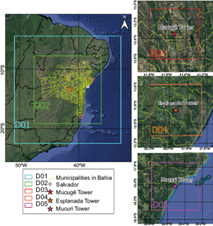
This study focuses on the state of Bahia, located in northeastern Brazil, between the parallels 08º 31’ 58” S and 18º 20’ 55” S, and the meridians 46º 37’ 02” W and 37º 20’ 28” W. The state of Bahia was the second largest producer of wind energy in Brazil in 2017 (7.79 TWh), behind only the state of Rio Grande do Norte (13.24 TWh). It also accounted for the second-highest factor average capacity in 2017 (48.5%), behind the state of Maranhão (68%) (ABEEólica, 2017). The interior of the state experiences the most intense winds concentrated in the dry period, unlike the conditions on the coast. Wind direction is observed to have little variation, with the east-west direction being predominant. Winds in the opposite direction are rarely recorded, and when recorded they exhibit very low speeds. The predominant climate is tropical, with high average temperatures and maximum annual temperatures above 30 ºC. In the hinterland, the climate is semi-arid, with annual rainfall below 800 mm. The rainy season is irregular, with prolonged drought events in the interior. The humidity on the coastal strip is higher than that in the interior and the annual accumulated precipitation exceeds 1600 mm in some regions (Camargo-Schubert, 2013). The generation of wind energy can vary in periods with more and less rain. In general, during periods of greatest drought (when it is not very windy), wind energy production suffers a small decrease. During the rainy periods (when there are more winds) there is a greater production of energy. Ramos et al. (2013) showed the influence of dry and rainy seasonality on energy behavior in the Northeast region of Brazil. Thus, analyses corresponding to the dry and rainy periods in each region are interesting, as the sites are very different from each other in terms of geographical position and seasonality.
The towers with anemometers are located at three different sites: the cities of Esplanada, Mucuri, and Mucugê. Table I show the summarized geographical information of the measurement sites.
Table I Geographical information of the measurement sites.
| Measurement sites | Latitude S | Longitude W |
| Esplanada Tower | 11º 50’ 55.22953” | 37º 55’ 44.31164” |
| Mucuri Tower | 18º 1’ 31.52” | 39º 30’ 51.69” |
| Mucugê Tower | 13º 21’ 01.9289” | 41º 31’ 53.76975” |
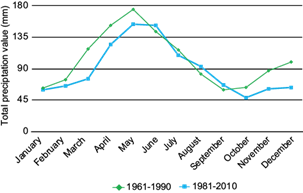
The city of Esplanada is located in the micro-region of the northern coast of Bahia at an altitude of 158 masl. Its anemometric tower is located 40 km from the sea. Analysis of the climatological normals (Fig. 1) available for the Alagoinhas station (closest to Esplanada) reveals that the months of December, January, February, September, and October are less rainy, while May and June are the rainiest months in this region.
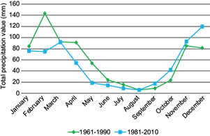
The city of Mucugê is situated at an altitude of 983 masl and is one of the municipalities belonging to Chapada Diamantina, the central region of the state of Bahia, characterized by its mountainous terrain. The Mucugê anemometric tower is located approximately 280 km from the coast of Bahia. Analysis of the climatological normals (Fig. 2) available for the Ituaçu station (closest to Mucugê) reveals that the months of May, June, July, August, and September are relatively dry, while November, December, January, and February are the rainiest months in this region.
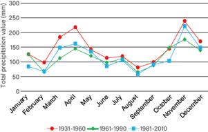
Finally, the city of Mucuri is located at an altitude of 7 masl. The Mucuri anemometric tower is located on a coastal plain, at a distance of 340 m from the sea. Analysis of the climatological normals (Fig. 3) available for the Caravelas station (closest to Mucuri) reveals that November, December, March, April, and May are the rainiest months in this region, while January, February, and August represent the driest period, considering the most current climatological normal (1981-2010).
3.2 Configuration of the WRF model
This study was conducted using the WRF meteorological model, version 3.9.1.1. The WRF model was configured using two nested domains with grid resolutions of 9 and 3 km, respectively. Inside the second domain, which covers the entire state of Bahia, three domains were designed with 1 km grid resolutions, centered on the three anemometric towers: Mucugê (Domain 3), Esplanada (Domain 4), and Mucuri (Domain 5). Figure 4 depicts the locations and distribution of domains in the WRF model. The domains were designed with horizontal dimensions of 223 × 223 and 420 × 420 grid cells corresponding to domains 1 and 2, respectively, and 60 × 60 grid cells corresponding to domains 3 to 5. During the initialization of WRF, data from the National Centers for Environmental Prediction (NCEP) Final Analysis (FNL), with a spatial resolution of 0.25º prepared operationally every 6 h were used (NCAR, 2015). Land use and occupation data were provided by the United States Geological Survey (USGS) with a resolution of 2’ corresponding to the largest domain and 30’’ corresponding to the others, which was made available to the default installation of the WRF model (Skamarock et al., 2008). The simulated winds were interpolated for heights of 80, 100, 120 and 150 m depending on the vertical profile of the WRF, based on hydrostatic pressure (ETA levels).
The simulations were carried out during December, 2015, and January, February, May, June, July, September, and October, 2016 (which are the months that have a representative percentage of observed data [> 75%] every hour). To obtain realistic initial conditions, a 24-hh spin-up was used, i.e., the simulation for each month was initialized from 00:00 UTC on the last day of the previous month. WRF outputs have been stored with hourly frequency, and the main model output parameters used were wind speed and direction.
The wind speed data acquisition was performed at three monitoring towers in the Bahia cities of Esplanada, Mucuri and Mucugê, as shown in Table I. The respective geographic locations are shown in Figure 4. Wind velocities are acquired by four anemometers located at different heights in the weather towers. The anemometers record a measurement at each level every 10 min and record an average every 60 min. The simulated data were also filtered in a similar way. The data was acquired using the Elipse E3 Supervisory Control and Data Acquisition (SCADA), which is a realtime SCADA platform for mission critical applications, being a well established SCADA platform, offering scalability and constant evolution for several types of applications, from simple HMI interfaces to complex operating centers in real time. It was developed to meet current and future connectivity the mean hourly values for the monitored data were computed. Suspicious or bad data (like negative values or a sequence of 20 or more equal-valued data) was treated as invalid data, which was discarded in order to produce valid samples. The anemometers are all Thies First Class.
3.3 Combinations of PBL and LSM schemes
The simulations tested the performances of all nine scenarios formed by the various combinations of three PBL schemes (MYJ, YSU, and ACM2) and three LSM schemes (Noah Land Surface Model [NLSM], RUC, and Noah-MP [multi-physics]), as presented in Table II. These PBL and LSM parameterization schemes were selected since they are the most common ones, as in the applications of Pei et al. (2014), Wharton et al. (2015), Lee et al. (2016), Salamanca et al. (2018), and Liu et al. (2019).
Table II Details of the test scenarios specifying the physical options.
| Scenarios | 1 | 2 | 3 | 4 | 5 | 6 | 7 | 8 | 9 |
| PBL | MYJ | MYJ | MYJ | YSU | YSU | YSU | ACM2 | ACM2 | ACM2 |
| Land surface model | NLSM | RUC | NOAH-MP | NLSM | RUC | NOAH-MP | NLSM | RUC | NOAH-MP |
| Surface layer | Eta | Eta | Eta | MM5 | MM5 | MM5 | MM5 | MM5 | MM5 |
| Cumulus | Kain-Fritsch | ||||||||
| Microphysics | WSM5 | ||||||||
| Shortwave radiation | Dudhia | ||||||||
| Longwave radiation | RRTM | ||||||||
PBL: planetary boundary layer; MYJ: Mellor-Yamada-Janjic PBL scheme; YSU: Yonsei University PBL scheme; ACM2: Asymmetric Convective Model 2; NLSM: Noah Land Surface Model; RUC: rapid update cycle; WSM5: the 5-class WRF single-moment; RRTM: Radiative Rapid Transfer Model.
The other parameterization schemes were maintained constant during the simulations. The 5-class WRF Single-Moment (WSM5) microphysics scheme (Hong et al., 2004) was chosen following Kitagawa et al. (2017), who studied the Metropolitan Region of Salvador (RMS) in the state of Bahia and obtained good estimates for the variables of wind speed and direction. The Radiative Rapid Transfer Model (RRTM) and the Dudhia scheme were selected to estimate long-wave and short-wave radiation due to their efficiency and satisfactory performance in studies of wind resources in various regions of the world (Amjad et al., 2015; Mattar and Borvoran, 2016; Giannaros et al., 2017; Argüeso and Businger, 2018). Convective processes were represented using the Kain-Fritsch cumulus scheme in the external domain, while it was disabled corresponding to other domains on the basis of the assumption that the majority of convective circulation is explicitly resolved. The physical options used are summarized in Table II, depicting the different scenarios.
3.4 Statistical evaluation
The performance of the model was evaluated using the statistical metrics of mean bias (MB), root mean squared error (RMSE), mean absolute gross error (MAGE), agreement index (IOA), and Pearson’s correlation coefficient (R) (Carvalho et al., 2012, 2014; Cheng et al., 2013; Zempila et al., 2016; Gunwani and Mohan, 2017; Surussavadee, 2017a, b). In addition, Factor of 2 (Fac2) (Zucatelli et al., 2019) and standard deviation (SD) (Penchah et al., 2017) were also used. The average error, also called the average bias, is defined as follows:
where M̅ denotes the modeled average and O̅ denotes the observed average.
Positive values of MB indicate an overestimation of the simulated data, while negative values imply underestimation. Positive/negative MB values corresponding to wind direction indicate that the modeled wind direction exhibits clockwise/counterclockwise overcorrection compared to the observations. It should be noted that, in the case of wind direction, the averages were calculated using scalar values and not vector values. The difference between each pair of simulated and observed wind directions (Δd) is defined as follows (Jiménez and Dudhia, 2013):
if,
if,
if,
The RMSE expresses the total error of the model and exhibits a value of zero in ideal cases.
In both of the aforementioned cases, lower values indicate better agreement between observed and modeled data. MAGE calculates the absolute mean error between simulated and observed values, expressing the average magnitude of the errors in the simulations.
As in the case of RMSE, lower values of MAGE indicate greater similarity between the observed and modeled data series. IOA evaluates how close the simulated value is to that observed. The metric ranges from -1 to 1, with the value “1” meaning perfect agreement. The term c is a constant relative to the model’s output frequency, which was assigned a value of 2 (Willmott et al., 2012). The variable P i corresponds to the simulated (“predicted”) value for instant (i), with O i indicating the value observed at the same time i and O̅ representing the average of the observed values.
Pearson’s correlation coefficient is a measure of linear association between modeled and observed data. Its value is zero in case of no correlation and the correlation increases as the value of the coefficient approaches -1 or +1. Values close to +1 imply positive correlation between the two variables, while those close to -1 imply negative correlation. It is defined as follows:
Factor of 2 (Fac2) calculates the ratio between the simulated (M i ) and observed (O i ) data, indicating the percentage of data that should lie within the range 0.5 ≤ M i / O i ≤ 2. Obviously, its value in the optimal case is 1.
4. Numerical results
Figure 5 depicts the average hourly time evolution of the observed and simulated wind speeds at elevations of 80, 100, 120, and 150 m, at the Mucuri, Esplanada, and Mucugê towers, obtained using the different combinations of PBL and LSM (see Table II). For the construction of hourly averages, all observed and simulated data records from the months studied were used.
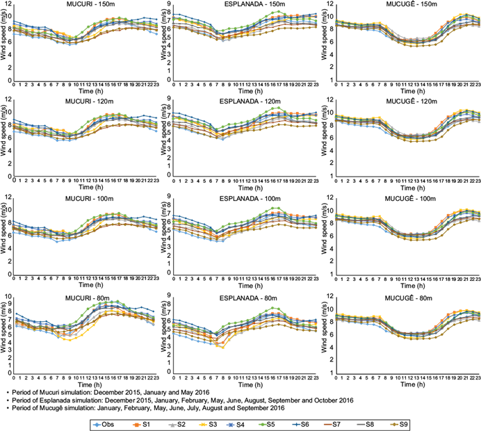
It is evident from Figure 5 that the simulated results typically closely follow the trend of the curve of the observed average hourly values. In particular, the data corresponding to Mucugê clearly exhibits a greater congruence between the simulated and observed curves. It is also verified that the values of the average hourly wind speeds vary approximately between 6 and 10 ms-1 at Mucuri and Mucugê, and between 3 and 8 ms-1 at Esplanada.
The analysis of the graphs in Figure 5 reveal a globally similar trend among the simulated scenarios, indicating that the model is capable of capturing the general behavior of the wind speed, despite small differences in terms of time and magnitude. In order to estimate the scenario that corresponds to the best performances, validation was performed based on the statistics evaluations. In this section, the statistical metrics (MB, RMSE, MAGE, IOA, R, Fac2 and SD) are analyzed in order to estimate the discrepancies between the simulated and observed wind speed and direction corresponding to each case.
Tables III, IV, and V present the values of the statistical metrics obtained by comparing the simulated and observed data on wind speed corresponding to the Mucuri, Esplanada, and Mucugê towers, respectively. Superior results have been highlighted in bold and, to evaluate simulations results, the objective hit Score (OhitS) (Penchah et al., 2017) was used. As mentioned previously, low values are better for MB, RMSE and MAGE, and high values are better for IOA, R, and Fac2 in terms of prediction accuracy. In the OhitS method, for SD, each parameterization that has the closest result to the corresponding observation gets an 8 score. The second-best parameterization gets a 7 score, and so on, the worst result gets a 0 score. For MB, RMSE and MAGE, parameterizations gain scores from 8 to 0 for minimum to maximum, respectively. For IOA, R and Fac2, the opposite occurs.
Table III Results of statistical metrics corresponding to the comparison between simulated and observed wind speed data at Mucuri tower.
| Height | S1 | S2 | S3 | S4 | S5 | S6 | S7 | S8 | S9 | Obs | |
| 150 m | MB | 0.846 | 0.454 | 0.742 | 0.854 | 0.885 | 1.024 | -0.131 | 0.406 | -0.227 | |
| OhitS | 3 | 5 | 4 | 2 | 1 | 0 | 8 | 6 | 7 | ||
| RMSE | 3.187 | 3.339 | 3.629 | 3.139 | 2.833 | 3.170 | 3.029 | 2.895 | 2.951 | ||
| OhitS | 2 | 1 | 0 | 4 | 8 | 3 | 5 | 7 | 6 | ||
| MAGE | 2.261 | 2.430 | 2.614 | 2.256 | 2.070 | 2.226 | 2.289 | 2.135 | 2.234 | ||
| OhitS | 3 | 1 | 0 | 4 | 8 | 6 | 2 | 7 | 5 | ||
| IOA | 0.512 | 0.475 | 0.436 | 0.513 | 0.553 | 0.511 | 0.506 | 0.539 | 0.517 | ||
| OhitS | 4 | 1 | 0 | 5 | 8 | 3 | 2 | 7 | 6 | ||
| R | 0.518 | 0.450 | 0.378 | 0.521 | 0.584 | 0.512 | 0.471 | 0.530 | 0.472 | ||
| OhitS | 5 | 1 | 0 | 6 | 8 | 4 | 2 | 7 | 3 | ||
| Fac2 | 87.8% | 85.9% | 85.3% | 88.7% | 89.1% | 88.1% | 87.1% | 88.7% | 87.2% | ||
| OhitS | 4 | 1 | 0 | 7 | 8 | 5 | 2 | 7 | 3 | ||
| SD | 3.413 | 3.449 | 3.457 | 3.440 | 3.229 | 3.341 | 3.161 | 3.146 | 2.954 | 2.849 | |
| OhitS | 3 | 1 | 0 | 2 | 5 | 4 | 6 | 7 | 8 | ||
| 120 m | MB | 0.781 | 0.425 | 0.653 | 0.747 | 0.786 | 0.915 | -0.169 | 0.341 | -0.266 | |
| OhitS | 2 | 5 | 4 | 3 | 1 | 0 | 8 | 6 | 7 | ||
| RMSE | 3.146 | 3.282 | 3.559 | 3.005 | 2.735 | 3.071 | 2.946 | 2.801 | 2.866 | ||
| OhitS | 2 | 1 | 0 | 4 | 8 | 3 | 5 | 7 | 6 | ||
| MAGE | 2.258 | 2.388 | 2.576 | 2.192 | 2.003 | 2.220 | 2.238 | 2.081 | 2.189 | ||
| OhitS | 2 | 1 | 0 | 5 | 8 | 4 | 3 | 7 | 6 | ||
| IOA | 0.507 | 0.478 | 0.437 | 0.521 | 0.563 | 0.515 | 0.511 | 0.545 | 0.522 | ||
| OhitS | 2 | 1 | 0 | 5 | 8 | 4 | 3 | 7 | 6 | ||
| R | 0.508 | 0.448 | 0.372 | 0.520 | 0.593 | 0.506 | 0.476 | 0.538 | 0.482 | ||
| OhitS | 5 | 1 | 0 | 6 | 8 | 4 | 2 | 7 | 3 | ||
| Fac2 | 86.9% | 85.5% | 84.4% | 88.4% | 88.6% | 87.8% | 86.0% | 88.4% | 86.9% | ||
| OhitS | 4 | 1 | 0 | 7 | 8 | 5 | 2 | 7 | 4 | ||
| SD | 3.308 | 3.349 | 3.345 | 3.230 | 3.126 | 3.175 | 3.025 | 3.022 | 2.834 | 2.859 | |
| OhitS | 2 | 0 | 1 | 3 | 5 | 4 | 6 | 7 | 8 | ||
| 100 m | MB | 0.649 | 0.368 | 0.485 | 0.668 | 0.726 | 0.823 | -0.158 | 0.330 | -0.259 | |
| OhitS | 3 | 5 | 4 | 2 | 1 | 0 | 8 | 6 | 7 | ||
| RMSE | 3.080 | 3.226 | 3.460 | 2.890 | 2.663 | 2.976 | 2.907 | 2.762 | 2.829 | ||
| OhitS | 2 | 1 | 0 | 5 | 8 | 3 | 4 | 7 | 6 | ||
| MAGE | 2.222 | 2.354 | 2.528 | 2.133 | 1.953 | 2.164 | 2.215 | 2.064 | 2.172 | ||
| OhitS | 2 | 1 | 0 | 6 | 8 | 5 | 3 | 7 | 4 | ||
| IOA | 0.513 | 0.484 | 0.446 | 0.532 | 0.572 | 0.526 | 0.514 | 0.547 | 0.524 | ||
| OhitS | 2 | 1 | 0 | 6 | 8 | 5 | 3 | 7 | 4 | ||
| R | 0.501 | 0.448 | 0.367 | 0.530 | 0.604 | 0.511 | 0.477 | 0.540 | 0.485 | ||
| OhitS | 4 | 1 | 0 | 6 | 8 | 5 | 2 | 7 | 3 | ||
| Fac2 | 86.0% | 85.2% | 83.7% | 88.5% | 88.7% | 87.4% | 85.8% | 88.6% | 86.9% | ||
| OhitS | 3 | 1 | 0 | 6 | 8 | 5 | 2 | 7 | 4 | ||
| SD | 3.203 | 3.256 | 3.201 | 3.089 | 3,070 | 3.058 | 2.947 | 2.954 | 2.769 | 2.866 | |
| OhitS | 1 | 0 | 2 | 3 | 4 | 5 | 8 | 7 | 6 | ||
| 80 m | MB | 0.071 | -0.245 | -0.431 | 0.577 | 0.667 | 0.714 | -0.142 | 0.322 | -0.251 | |
| OhitS | 8 | 6 | 3 | 2 | 1 | 0 | 7 | 4 | 5 | ||
| RMSE | 2.540 | 2.685 | 2.835 | 2.767 | 2.593 | 2.865 | 2.858 | 2.717 | 2.783 | ||
| OhitS | 8 | 6 | 1 | 4 | 7 | 0 | 2 | 5 | 3 | ||
| MAGE | 1.914 | 2.058 | 2.172 | 2.058 | 1.913 | 2.091 | 2.187 | 2.043 | 2.146 | ||
| OhitS | 7 | 5 | 1 | 5 | 8 | 3 | 2 | 6 | 0 | ||
| IOA | 0.580 | 0.549 | 0.524 | 0.549 | 0.581 | 0.542 | 0.521 | 0.552 | 0.530 | ||
| OhitS | 7 | 5 | 1 | 5 | 8 | 3 | 0 | 6 | 2 | ||
| R | 0.585 | 0.540 | 0.483 | 0.547 | 0.616 | 0.524 | 0.483 | 0.546 | 0.493 | ||
| OhitS | 7 | 4 | 1 | 5 | 8 | 3 | 1 | 6 | 2 | ||
| Fac2 | 87.3% | 86.7% | 84.3% | 88.3% | 88.7% | 86.8% | 85.1% | 87.5% | 86.7% | ||
| OhitS | 5 | 3 | 0 | 7 | 8 | 4 | 1 | 6 | 3 | ||
| SD | 2.827 | 2.808 | 2.690 | 2.968 | 3.029 | 2.951 | 2.873 | 2.894 | 2.710 | 2.876 | |
| OhitS | 6 | 5 | 0 | 3 | 2 | 4 | 8 | 7 | 1 | ||
| Sum of scores | 108 | 65 | 22 | 128 | 179 | 94 | 107 | 184 | 128 | ||
MB: mean bias; RMSE: root mean squared error; MAGE: mean absolute gross error; IOA: agreement index; R: Pearson’s correlation coefficient; Fac2: Factor of 2; SD: standard deviation; Ohits: objective hit score; S: station; Obs: observed. The best results are highlighted in bold.
Table IV Results of statistical metrics corresponding to the comparison between simulated and observed wind speed data at Esplanada tower.
| Height | S1 | S2 | S3 | S4 | S5 | S6 | S7 | S8 | S9 | Obs | |
| 150 m | MB | 0.613 | -0.160 | 0.292 | 0.614 | 0.730 | 0.737 | -0.171 | 0.152 | -0.506 | |
| OhitS | 3 | 7 | 5 | 2 | 1 | 0 | 6 | 8 | 4 | ||
| RMSE | 2.007 | 2.193 | 1.934 | 2.098 | 1.898 | 2.029 | 2.151 | 1.990 | 2.074 | ||
| OhitS | 5 | 0 | 7 | 2 | 8 | 4 | 1 | 6 | 3 | ||
| MAGE | 1.448 | 1.679 | 1.486 | 1.574 | 1.453 | 1.521 | 1.673 | 1.491 | 1.625 | ||
| OhitS | 7 | 0 | 6 | 3 | 8 | 4 | 1 | 5 | 2 | ||
| IOA | 0.446 | 0.384 | 0.455 | 0.423 | 0.467 | 0.442 | 0.386 | 0.453 | 0.404 | ||
| OhitS | 5 | 0 | 7 | 3 | 8 | 4 | 1 | 6 | 2 | ||
| R | 0.492 | 0.409 | 0.465 | 0.509 | 0.530 | 0.511 | 0.398 | 0.423 | 0.400 | ||
| OhitS | 5 | 2 | 4 | 6 | 8 | 7 | 0 | 3 | 1 | ||
| Fac2 | 93.9% | 88.9% | 93.2% | 93.1% | 94.6% | 94.2% | 89.6% | 92.2% | 90.1% | ||
| OhitS | 6 | 0 | 5 | 4 | 8 | 7 | 1 | 3 | 2 | ||
| SD | 2.133 | 2.242 | 1.976 | 2.245 | 1.912 | 2.068 | 2.154 | 1.980 | 1.961 | 1.708 | |
| OhitS | 3 | 1 | 6 | 0 | 8 | 4 | 2 | 5 | 7 | ||
| 120 m | MB | 0.721 | -0.026 | 0.378 | 0.752 | 0.824 | 0.831 | -0,003 | 0.319 | -0.372 | |
| OhitS | 3 | 7 | 4 | 2 | 1 | 0 | 8 | 6 | 5 | ||
| RMSE | 2.062 | 2.174 | 1.993 | 2.138 | 1.934 | 2.081 | 2.115 | 1.992 | 2.023 | ||
| OhitS | 4 | 0 | 6 | 1 | 8 | 3 | 2 | 7 | 5 | ||
| MAGE | 1.540 | 1.668 | 1.535 | 1.609 | 1.486 | 1.576 | 1.648 | 1.493 | 1.586 | ||
| OhitS | 5 | 0 | 6 | 2 | 8 | 4 | 1 | 7 | 3 | ||
| IOA | 0.434 | 0.389 | 0.438 | 0.411 | 0.456 | 0.423 | 0.396 | 0.453 | 0.419 | ||
| OhitS | 5 | 0 | 6 | 2 | 8 | 4 | 1 | 7 | 3 | ||
| R | 0.476 | 0.400 | 0.438 | 0.489 | 0.520 | 0.480 | 0.390 | 0.408 | 0.391 | ||
| OhitS | 5 | 2 | 4 | 7 | 8 | 6 | 0 | 3 | 1 | ||
| Fac2 | 92.4% | 87.5% | 91.8% | 91.5% | 93.2% | 92.2% | 88.3% | 90.7% | 88.9% | ||
| OhitS | 7 | 0 | 5 | 4 | 8 | 6 | 1 | 3 | 2 | ||
| SD | 2.115 | 2.208 | 1.975 | 2.186 | 1.877 | 2.009 | 2.097 | 1.917 | 1.906 | 1.700 | |
| OhitS | 2 | 0 | 5 | 1 | 8 | 4 | 3 | 6 | 7 | ||
| 100 m | MB | 0.750 | 0.049 | 0.354 | 0.833 | 0.882 | 0.869 | 0.134 | 0.456 | -0.251 | |
| OhitS | 3 | 8 | 5 | 2 | 0 | 1 | 7 | 4 | 6 | ||
| RMSE | 2.078 | 2.139 | 2.010 | 2.148 | 1.954 | 2.101 | 2.076 | 1.989 | 1.978 | ||
| OhitS | 3 | 1 | 5 | 0 | 8 | 2 | 4 | 6 | 7 | ||
| MAGE | 1.557 | 1.651 | 1.547 | 1.623 | 1.504 | 1.598 | 1.617 | 1.492 | 1.551 | ||
| OhitS | 4 | 0 | 6 | 1 | 7 | 3 | 2 | 8 | 5 | ||
| IOA | 0.436 | 0.403 | 0.441 | 0.413 | 0.456 | 0.422 | 0.416 | 0.461 | 0.439 | ||
| OhitS | 4 | 0 | 6 | 1 | 7 | 3 | 2 | 8 | 5 | ||
| R | 0.473 | 0.404 | 0.422 | 0.486 | 0.527 | 0.466 | 0.401 | 0.416 | 0.399 | ||
| OhitS | 6 | 2 | 4 | 7 | 8 | 5 | 1 | 3 | 0 | ||
| Fac2 | 90.6% | 86.1% | 90.1% | 89.4% | 91.4% | 90.5% | 87.4% | 89.6% | 88.0% | ||
| OhitS | 7 | 0 | 5 | 3 | 8 | 6 | 1 | 4 | 2 | ||
| SD | 2.109 | 2.161 | 1.956 | 2.139 | 1.877 | 1.969 | 2.053 | 1.878 | 1.871 | 1.713 | |
| OhitS | 2 | 0 | 5 | 1 | 7 | 4 | 3 | 6 | 8 | ||
| 80 m | MB | 0.606 | -0.022 | 0.120 | 0.829 | 0.880 | 0.824 | 0.202 | 0.533 | -0.184 | |
| OhitS | 3 | 8 | 7 | 1 | 0 | 2 | 5 | 4 | 6 | ||
| RMSE | 1.990 | 2.055 | 1.898 | 2.092 | 1.935 | 2.062 | 2.033 | 1.975 | 1.942 | ||
| OhitS | 4 | 1 | 8 | 0 | 7 | 2 | 3 | 5 | 6 | ||
| MAGE | 1.495 | 1.593 | 1.476 | 1.589 | 1.489 | 1.572 | 1.583 | 1.488 | 1.524 | ||
| OhitS | 5 | 0 | 8 | 1 | 6 | 3 | 2 | 7 | 4 | ||
| IOA | 0.482 | 0.447 | 0.488 | 0.449 | 0.484 | 0.455 | 0.451 | 0.484 | 0.471 | ||
| OhitS | 5 | 0 | 8 | 1 | 7 | 3 | 2 | 7 | 4 | ||
| R | 0.494 | 0.433 | 0.454 | 0.503 | 0.554 | 0.473 | 0.431 | 0.446 | 0.423 | ||
| OhitS | 6 | 2 | 4 | 7 | 8 | 5 | 1 | 3 | 0 | ||
| Fac2 | 88.8% | 84.9% | 88.3% | 87.7% | 90.0% | 88.5% | 86.1% | 88.5% | 87.0% | ||
| OhitS | 7 | 0 | 4 | 3 | 8 | 6 | 1 | 6 | 2 | ||
| SD | 2.067 | 2.081 | 1.868 | 2.067 | 1.891 | 1.913 | 2.017 | 1.859 | 1.845 | 1.770 | |
| OhitS | 1 | 0 | 6 | 2 | 5 | 4 | 3 | 7 | 8 | ||
| Sum of scores | 125 | 41 | 157 | 69 | 184 | 106 | 65 | 153 | 110 | ||
MB: mean bias; RMSE: root mean squared error; MAGE: mean absolute gross error; IOA: agreement index; R: Pearson’s correlation coefficient; Fac2: Factor of 2; SD: standard deviation; Ohits: objective hit score; S: station; Obs: observed. The best results are highlighted in bold.
Table V Results of statistical metrics corresponding to the comparison between simulated and observed wind speed data at Mucugê tower.
| Height | S1 | S2 | S3 | S4 | S5 | S6 | S7 | S8 | S9 | Obs | |
| 150 m | MB | 0.700 | 0.364 | 0.698 | 0.420 | 0.519 | 0.528 | 0.138 | 0.159 | -0.289 | |
| OhitS | 0 | 5 | 1 | 4 | 3 | 2 | 8 | 7 | 6 | ||
| RMSE | 2.932 | 3.237 | 2.857 | 2.682 | 2.567 | 2.496 | 2.874 | 2.781 | 2.622 | ||
| OhitS | 1 | 0 | 3 | 5 | 7 | 8 | 2 | 4 | 6 | ||
| MAGE | 2.280 | 2.559 | 2.229 | 2.144 | 2.026 | 1.943 | 2.272 | 2.197 | 2.088 | ||
| OhitS | 2 | 0 | 3 | 5 | 7 | 8 | 1 | 4 | 6 | ||
| IOA | 0.450 | 0.409 | 0.485 | 0.505 | 0.532 | 0.552 | 0.476 | 0.493 | 0.519 | ||
| OhitS | 1 | 0 | 3 | 5 | 7 | 8 | 2 | 4 | 6 | ||
| R | 0.614 | 0.519 | 0.619 | 0.649 | 0.650 | 0.662 | 0.598 | 0.609 | 0.621 | ||
| OhitS | 2 | 0 | 4 | 6 | 7 | 8 | 1 | 3 | 5 | ||
| Fac2 | 88.4% | 84.1% | 88.8% | 89.2% | 91.5% | 92.3% | 86.2% | 87.4% | 87.7% | ||
| OhitS | 4 | 0 | 5 | 6 | 7 | 8 | 1 | 2 | 3 | ||
| SD | 3.700 | 3.650 | 3.491 | 3.467 | 3.275 | 3.220 | 3.536 | 3.448 | 3.253 | 2.691 | |
| OhitS | 0 | 1 | 3 | 4 | 6 | 8 | 2 | 5 | 7 | ||
| 120 m | MB | 0.857 | 0.440 | 0.812 | 0.581 | 0.647 | 0.640 | 0.311 | 0.321 | -0.169 | |
| OhitS | 0 | 5 | 1 | 4 | 2 | 3 | 7 | 6 | 8 | ||
| RMSE | 2.915 | 3.184 | 2.842 | 2.654 | 2.547 | 2.486 | 2.829 | 2.745 | 2.559 | ||
| OhitS | 1 | 0 | 2 | 5 | 7 | 8 | 3 | 4 | 6 | ||
| MAGE | 2.255 | 2.513 | 2.216 | 2.113 | 2.004 | 1.934 | 2.229 | 2.160 | 2.029 | ||
| OhitS | 1 | 0 | 3 | 5 | 7 | 8 | 2 | 4 | 6 | ||
| IOA | 0.440 | 0.402 | 0.473 | 0.498 | 0.523 | 0.540 | 0.470 | 0.486 | 0.517 | ||
| OhitS | 1 | 0 | 2 | 5 | 7 | 8 | 3 | 4 | 6 | ||
| R | 0.600 | 0.502 | 0.602 | 0.639 | 0.640 | 0.648 | 0.558 | 0.596 | 0.607 | ||
| OhitS | 3 | 0 | 4 | 6 | 7 | 8 | 1 | 2 | 5 | ||
| Fac2 | 89.0% | 84.1% | 88.6% | 89.6% | 91.5% | 92.4% | 86.9% | 88.2% | 88.6% | ||
| OhitS | 5 | 0 | 4 | 6 | 7 | 8 | 1 | 2 | 4 | ||
| SD | 3.567 | 3.523 | 3.366 | 3.336 | 3.158 | 3.097 | 3.421 | 3.328 | 3.123 | 2.605 | |
| OhitS | 0 | 1 | 3 | 4 | 6 | 8 | 2 | 5 | 7 | ||
| 100 m | MB | 0.779 | 0.306 | 0.692 | 0.517 | 0.553 | 0.517 | 0.264 | 0.261 | -0.262 | |
| OhitS | 0 | 5 | 1 | 4 | 2 | 4 | 6 | 8 | 7 | ||
| RMSE | 2.864 | 3.142 | 2.793 | 2.620 | 2.507 | 2.435 | 2.811 | 2.728 | 2.557 | ||
| OhitS | 1 | 0 | 3 | 5 | 7 | 8 | 2 | 4 | 6 | ||
| MAGE | 2.210 | 2.473 | 2.172 | 2.079 | 1.963 | 1.891 | 2.209 | 2.143 | 2.033 | ||
| OhitS | 1 | 0 | 3 | 5 | 7 | 8 | 2 | 4 | 6 | ||
| IOA | 0.450 | 0.412 | 0.483 | 0.506 | 0.533 | 0.550 | 0.475 | 0.491 | 0.517 | ||
| OhitS | 1 | 0 | 3 | 5 | 7 | 8 | 2 | 4 | 6 | ||
| R | 0.584 | 0.484 | 0.585 | 0.624 | 0.627 | 0.636 | 0.572 | 0.578 | 0.590 | ||
| OhitS | 3 | 0 | 4 | 6 | 7 | 8 | 1 | 2 | 5 | ||
| Fac2 | 89.4% | 84.4% | 88.8% | 90.1% | 91.8% | 92.7% | 87.3% | 88.6% | 89.0% | ||
| OhitS | 5 | 0 | 3 | 6 | 7 | 8 | 1 | 2 | 4 | ||
| SD | 3.449 | 3.408 | 3.261 | 3.222 | 3.053 | 2.979 | 3.323 | 3.224 | 3.017 | 2.607 | |
| OhitS | 0 | 1 | 3 | 5 | 6 | 8 | 2 | 4 | 7 | ||
| 80 m | MB | 0.736 | 0.209 | 0.582 | 0.499 | 0.503 | 0.417 | 0.268 | 0.246 | -0.307 | |
| OhitS | 0 | 8 | 1 | 3 | 2 | 4 | 6 | 7 | 5 | ||
| RMSE | 2.786 | 3.056 | 2.703 | 2.589 | 2.475 | 2.376 | 2.794 | 2.708 | 2.547 | ||
| OhitS | 2 | 0 | 4 | 5 | 7 | 8 | 1 | 3 | 6 | ||
| MAGE | 2.145 | 2.408 | 2.099 | 2.047 | 1.928 | 1.843 | 2.188 | 2.123 | 2.025 | ||
| OhitS | 2 | 0 | 4 | 5 | 7 | 8 | 1 | 3 | 6 | ||
| IOA | 0.454 | 0.416 | 0.491 | 0.503 | 0.532 | 0.553 | 0.469 | 0.485 | 0.509 | ||
| OhitS | 1 | 0 | 4 | 5 | 7 | 8 | 2 | 3 | 6 | ||
| R | 0.567 | 0.466 | 0.568 | 0.605 | 0.609 | 0.620 | 0.548 | 0.554 | 0.566 | ||
| OhitS | 4 | 0 | 5 | 6 | 7 | 8 | 1 | 2 | 3 | ||
| Fac2 | 89.7% | 84.9% | 88.8% | 90.3% | 91.5% | 92.6% | 87.3% | 88.7% | 89.1% | ||
| OhitS | 5 | 0 | 3 | 6 | 7 | 8 | 1 | 2 | 4 | ||
| SD | 3.285 | 3.245 | 3.097 | 3.093 | 2.936 | 2.836 | 3.204 | 3.099 | 2.892 | 2.557 | |
| OhitS | 0 | 1 | 4 | 5 | 6 | 8 | 2 | 3 | 7 | ||
| Sum of scores | 46 | 27 | 86 | 141 | 173 | 205 | 66 | 107 | 159 | ||
MB: mean bias; RMSE: root mean squared error; MAGE: mean absolute gross error; IOA: agreement index; R: Pearson’s correlation coefficient; Fac2: Factor of 2; SD: standard deviation; Ohits: objective hit score; S: station; Obs: observed. The best results are highlighted in bold.
Based on the comparison between measurements obtained in the three towers, the common parameterization with the highest score was obtained by scenario 5 (S5) (parameterization YSU and RUC): 184 points in Esplanada, 179 points in Mucuri, and 173 points in Mucugê. In the meantime, scenario 6 (S6) showed the best performance corresponding to Mucugê (parameterizations YSU and NOAH-MP). However, the results obtained by this scenario were as good as those obtained by scenario 5 in all cases. The underestimation of wind speed only occurred in the simulations performed with ACM2-Noah-MP for all levels and towers, and with ACM2-LSM at all levels for Mucuri and at 120 and 150 m in height for Esplanada. Tyagi et al. (2018) also found that ACM2 underestimated wind speed, while MYJ and YSU overestimated this parameter.
These metrics were also evaluated corresponding to the variable of wind direction. Corresponding to Mucugê, as in the case of wind speed, the combination of the YSU scheme and the NOAH-MP soil surface scheme (S6) produced the best estimates. However, Esplanada and Mucuri exhibited different results compared to the case of wind speed. Corresponding to Mucuri, the combination of MYJ atmospheric boundary layer parameterization and the Noah (S1) model performed better overall compared to other combinations. Finally, corresponding to Esplanada, scenario 3 (S3), which comprises the combination of MYJ and NOAH-MP, obtained a better result than the other combinations.
From the perspective of wind energy, wind speed is a more important variable than wind direction. This can be primarily attributed to the existence of a system that guides the wind turbine rotor in the direction of the wind and the automatic regulation of the slopes of the blades to optimize the incidence of wind. Thus, the results obtained from the analysis of wind speed is more pertinent to simulations with high resolution domain for the entire state of Bahia, given that it produces a high amount of wind energy. Based on the aforementioned discussion, further analyses of the parametrization performance of the combination of the CLP-YSU and LSM-RUC schemes in terms of wind speed follow.
Figures 6, 7, and 8 illustrate the wind roses obtained using YSU and RUC (scenario 5) as parameterizations of PBL and LSM, respectively, corresponding to the three towers: Mucuri (Fig. 6), Esplanada (Fig. 7) and Mucugê (Fig. 8), based on all data generated during the simulated months.
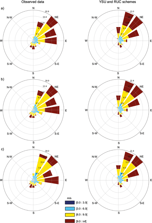
Fig. 6 Comparison of wind roses obtained using the YSU and RUC schemes from the Mucuri tower based on observations at heights of (a) 150 m, (b) 120 m, and (c) 100 m.
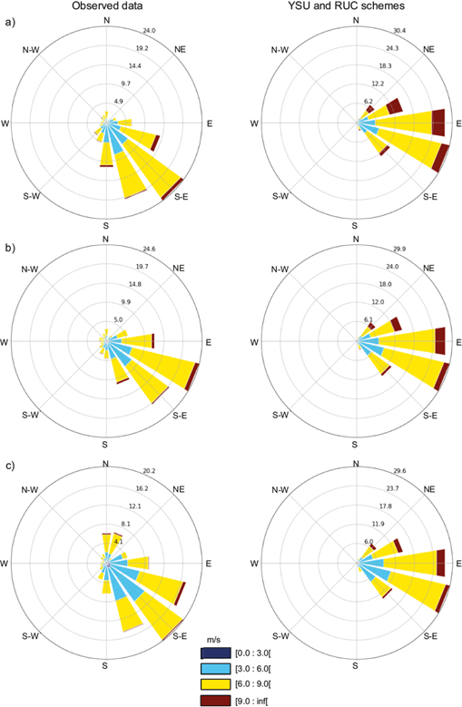
Fig. 7 Comparison of wind roses obtained using the YSU and RUC schemes from the Esplanada tower based on observations at heights of (a) 150 m, (b) 120 m, and (c) 100 m.
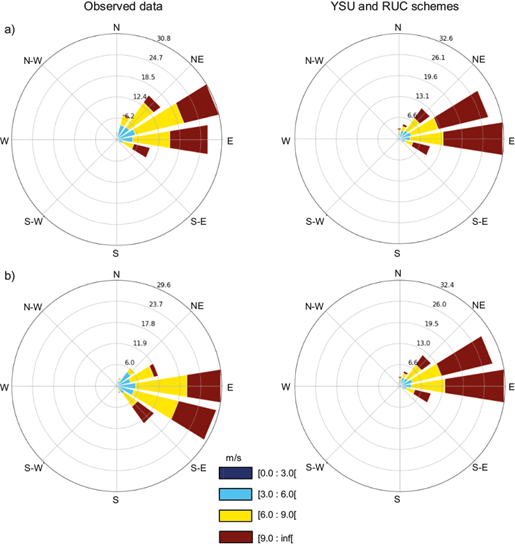
Fig. 8 Comparison of wind roses obtained using the YSU and RUC schemes from the Mucugê tower based on observations at heights of (a) 120 m, and (b) 100 m.
It is evident from the wind rose diagrams that the studied regions exhibit high potential for wind power generation with intermediate and high wind speed values between 6 to 9 ms-1 (yellow) and above 9 ms-1 (brown), respectively. It is also apparent that the wind speed was slightly overestimated at all three towers. This agrees with the observations of Giannaros et al. (2017), who highlighted the tendency of the WRF model to overestimate the frequency of strong winds; Stucki et al. (2016), who reported that the WRF model tends to overestimate average winds; and Carvalho et al. (2014), who also reported similar results.
As this study uses data from towers located at three different sites equipped with anemometers at varying heights (80, 100, 120 and 150 m), its observations can be considered to be representative in terms of wind energy. Thus, it is interesting to compare these data with the vertical profiles of wind obtained via the simulations. Figures 9, 10, and 11 depict the vertical profiles of the monthly average wind speeds simulated using scenario 5 (YSU and RUC), for two representative months each corresponding to the dry and rainy periods, compared to data observed at the Esplanada, Mucugê, and Mucuri towers, respectively. Table VI specifies the two representative months for dry and rainy periods for each tower.
Fig. 9 Vertical profiles of the monthly average wind speed measured by the Esplanada tower and simulated using WRF with the parameters of scenario 5 in (a) January, and (b) May.
Fig. 10 Vertical profiles of the monthly average wind speed measured by the Mucugê tower and simulated using WRF with the parameterization of scenario 5 in (a) January, and (b) July.
Fig. 11 Vertical profiles of the monthly average wind speed measured by the Mucuri tower and simulated using WRF with the parameterization of scenario 5 in (a) January, and (b) May.
Table VI Representative months for dry and rainy periods for each tower.
| Esplanada | Mucuri | Mucugê | ||
| Month | Rainy | May | May | January |
| Dry | January | January | July |
Data corresponding to Esplanada is observed to be well characterized with two very distinct periods and abundant rain during the months of May and June (see Fig. 1). The average monthly speed is overestimated by the WRF model at all heights during May (Fig. 9b); however, the maximum difference between simulated and observed data is observed to be 0.64 ms-1. During the less rainy period in January, the difference is observed to be 1.34 ms-1 and the tendency of overestimation is also observed (Fig. 9a).
Data corresponding to Mucugê (the farthest from the sea) is also well characterized with two very distinct periods and very little rain during the months of July and August (see Fig. 2). The average monthly speed is overestimated by the WRF model at all heights during July, with a maximum difference of 1.34 ms-1 (Fig. 10b). During the rainiest period in January, the maximum difference is observed to be 0.22 ms-1, but a slight tendency of overestimation persists (Fig. 10a).
Data corresponding to Mucuri (the closest to the sea) has been uniform in terms of annual rainfall over the most recent decades (see Fig. 3); however, January and February are representative of the dry season in the region. During this period, the average monthly speed is overestimated by the WRF model at all heights during January, with a maximum difference of 1.66 ms-1 (Fig. 11a). During May, which is representative of the rainy season in the region, the maximum difference is observed to be 0.27 ms-1 (Fig. 11b).
Therefore, consideration of only the months analyzed disaggregated from the others reveals a greater tendency of overestimation of the monthly average wind speed corresponding to the dry season.
Having identified the best performing combination to be the YSU-RUC scheme, the superiority of its performance can be verified with respect to each location, in terms of the distance from the sea (Table VII), based on the evaluated statistics corresponding to all the simulated months. Unlike tables III, IV and V that compare 9 scenarios, in table VII the three towers are compared, therefore, the scores ranged between 2 and 0. SD was analyzed by the difference between simulated and observed SD (diffSD).
Table VII Wind speed statistics obtained using the YSU and RUC schemes.
| Height | Esplanada | Mucuri | Mucugê | |
| 150 m | MB | 0.730 | 0.885 | 0.519 |
| OhitS | 1 | 0 | 2 | |
| RMSE | 1.898 | 2.833 | 2.567 | |
| OhitS | 2 | 0 | 1 | |
| MAGE | 1.453 | 2.070 | 2.026 | |
| OhitS | 2 | 0 | 1 | |
| IOA | 0.467 | 0.553 | 0.532 | |
| OhitS | 0 | 2 | 1 | |
| R | 0.530 | 0.584 | 0.650 | |
| OhitS | 0 | 1 | 2 | |
| Fac2 | 94.6% | 89.1% | 91.5% | |
| OhitS | 2 | 0 | 1 | |
| diffSD | 0.204 | 0.379 | 0.584 | |
| OhitS | 2 | 1 | 0 | |
| 120 m | MB | 0.824 | 0.786 | 0.647 |
| OhitS | 0 | 1 | 2 | |
| RMSE | 1.934 | 2.735 | 2.547 | |
| OhitS | 2 | 0 | 1 | |
| MAGE | 1.486 | 2.003 | 2.004 | |
| OhitS | 2 | 1 | 0 | |
| IOA | 0.456 | 0.563 | 0.523 | |
| OhitS | 0 | 2 | 1 | |
| R | 0.520 | 0.593 | 0.640 | |
| OhitS | 0 | 1 | 2 | |
| Fac2 | 93.2% | 88.6% | 91.5% | |
| OhitS | 2 | 0 | 1 | |
| diffSD | 0.177 | 0.267 | 0.552 | |
| OhitS | 2 | 1 | 0 | |
| Height | Esplanada | Mucuri | Mucugê | |
| 100 m | MB | 0.882 | 0.726 | 0.553 |
| OhitS | 0 | 1 | 2 | |
| RMSE | 1.954 | 2.663 | 2.507 | |
| OhitS | 2 | 0 | 1 | |
| MAGE | 1.504 | 1.953 | 1.963 | |
| OhitS | 2 | 1 | 0 | |
| IOA | 0.456 | 0.572 | 0.533 | |
| OhitS | 0 | 2 | 1 | |
| R | 0.527 | 0.604 | 0.627 | |
| OhitS | 0 | 1 | 2 | |
| Fac2 | 91.4% | 88.7% | 91.8% | |
| OhitS | 1 | 0 | 2 | |
| diffSD | 0.164 | 0.204 | 0.447 | |
| OhitS | 2 | 1 | 0 | |
| 80 m | MB | 0.880 | 0.667 | 0.503 |
| OhitS | 0 | 1 | 2 | |
| RMSE | 1.935 | 2.593 | 2.475 | |
| OhitS | 2 | 0 | 1 | |
| MAGE | 1.489 | 1.913 | 1.928 | |
| OhitS | 2 | 1 | 0 | |
| IOA | 0.484 | 0.581 | 0.532 | |
| OhitS | 0 | 2 | 1 | |
| R | 0.554 | 0.616 | 0.609 | |
| OhitS | 0 | 2 | 1 | |
| Fac2 | 90.0% | 88.7% | 91.5% | |
| OhitS | 1 | 0 | 2 | |
| diffSD | 0.122 | 0.152 | 0.379 | |
| OhitS | 2 | 1 | 0 | |
| Sum of scores | 31 | 23 | 30 | |
MB: mean bias; RMSE: root mean squared error; MAGE: mean absolute gross error; IOA: agreement index; R: Pearson’s correlation coefficient; Fac2: Factor of 2; SD: standard deviation; Ohits: objective hit score; S: station; Obs: observed. The best results are highlighted in bold.
An analysis of Table VII and Figure 5 reveals that proximity to the sea degrades the accuracy of simulation. Mucugê is observed to exhibit a greater congruence between simulated and observed wind speeds (Fig. 5). This tower, located in the center of the state of Bahia (280 km from the sea), exhibits a statistically similar performance to that at Esplanada (40 km from the coast), and corresponds to a better performance than that recorded at Mucuri (tower closest to the sea, 340 m). This phenomenon can be explained by the differentiated behavior of the model in regions close to large bodies of water compared to more inland areas. At places near the sea, variations in atmospheric conditions are more localized in time and space, due to ill-understood effects of land and sea breezes that are not accounted for by atmospheric models (Salvador et al., 2016b). Proximity to the sea, the interactions between atmospheric flow in the marine boundary layer, and the development of a boundary layer on the continent remain critical factors in the predictions of such models. Further, the adequate simulation of the flow characteristics related to the breeze inlet marine life in coastal regions persists as one of the major challenges for meteorological models (Shin e Hong, 2011; Cheng et al., 2012; de León and Orfila, 2013). It should be noted that the model interpreted the grid cell containing the Mucuri tower as land, which refutes the hypothesis that its poor performance is induced by the mistaken identification of the site as oceanic (given its close proximity to the sea), and supports the hypothesis that proximity to the sea negatively influences the performance of simulations. Tyagi et al. (2018) found a similar result by indicating that inland locations are better simulated than sea locations, and indicated the reasons for this difference in the fact that performance is likely related to difficulty in reproducing vertical variability at sea, where very shallow PBL development may not be entirely reproduced. In addition, simulated PBL depths at sea locations exhibit a larger bias with respect to observations at inland locations with well-developed convective boundary layers.
Assessment of the wind speed statistics corresponding to periods of more and less rain also reveals scenario 5 (YSU and RUC) to be well-performing. It is interesting to note that the most accurate estimates for wind speed corresponding to the period of less rain in the simulated months in Mucugê (May, June, July, and September), were identical to the one obtained via aggregate analysis (parameterizations YSU and NOAH-MP [S6]). Analysis of the rainy period (January and February) also revealed better estimates corresponding to scenario 5 (YSU and RUC). Following the disaggregation of the two periods (more and less rain) at Esplanada, the data corresponding to the least rainy period (December, January, February, September, and October) continued to support the finding that scenario 5 exhibited the best performance, while better indicators were obtained corresponding to the rainy period (May and June) using scenario 1 (MYJ and NLSM). Corresponding to Mucuri, scenario 5 (YSU and RUC) continued to emerge as the best option for the drier month (January), while the rainy months (December and May) were better characterized by scenario 8 (ACM2 and RUC). However, the results obtained by these scenarios were as good as those obtained by scenario 5 in all cases. Thus, the aforementioned results corroborate the choice of the combination of the PBL-YSU scheme with the LSM-RUC scheme for application in the forecast of wind energy production for the region.
5. Summary and conclusions
This study aimed to evaluate the performance of the various combinations of three PBL parameterization schemes and three LSM parameterization schemes, using the WRF model for a tropical region, in order to identify the optimal parameters to be applied in the analysis of wind energy production based on numerical modeling.
The WRF model was verified to be capable of capturing the general behavior of wind speed. The combination of the YSU and RUC parameterization schemes exhibited the best performance. As expected, the simple scheme of thermal diffusion of the soil, RUC, was better adapted to the case of Bahia, as this region does not experience snowy climate. The RUC scheme was also observed to fit into the intermediate level of complexity.
It is important to highlight that wind speed was overestimated in the simulations and, in general, estimated wind directions were quite similar to the observed data. Further, it was observed that proximity to the ocean degraded the accuracy of the simulations. Thus, the towers at Mucugê and Esplanada, which were farthest from the sea, exhibited the best results for all statistical metrics with respect to wind speed. However, the average hourly time evolution of observed and simulated wind speeds at Mucugê exhibited less dissonance.
Finally, the disaggregated analysis of the results corresponding to rainy and dry periods at each tower revealed YSU-RUC to be the clear front-runner. This fact supports the application of the combination of CLP-YSU and LSM-RUC to the high-resolution simulation of wind energy production for the entire state of Bahia. This should be the next step in order to obtain a high-resolution wind map with verified parameterization that exhibits good results.

