nueva página del texto (beta)
 Inglés (pdf)
 Artículo en XML
 Referencias del artículo
 Enviar artículo por email
 Citado por SciELO
  Similares en
SciELO
Similares en
SciELO 
 Permalink
1. Introduction
Inefficient use of fuels and energy processes in growing urban areas are associated with poor air quality, which has important implications on health and climate change at local, regional, and global scales. The region in central Mexico known as El Bajío, with a population of approximately 20 million, is a major center of economic activity that includes large, industrialized cities such as Guadalajara, León, Querétaro, and Aguascalientes, as well as the Salamanca refinery. Manufacturing and transportation are probably the most important anthropogenic activities with emissions to the atmosphere in this region (INEGI, 2015). Air quality in the main cities of El Bajío is often reported as bad; however, there is a lack of understanding of the origin (emissions and transport) of air pollutants in this region despite its large population and economic relevance (INECC, 2019). Without such knowledge, policy makers cannot develop environmental and economic policies leading to a more orderly planning and sustainable growth, and to improvements in air quality, protection of public health, and mitigation of the effects of climate change.
The Metropolitan Area of Querétaro (MAQ) located 200 km north of Mexico City on the southeast border of El Bajío, is one of the fastest growing urban areas in Mexico, with a population of 1.3 million in 2015. In addition to local industry and traffic, the MAQ is surrounded by important area sources such as the industrial corridor León-Irapuato-Salamanca, where the Salamanca refinery is located. Little is understood about the interactions between emissions, air quality, and climate in the MAQ and El Bajío, and it is unclear how regional sources of emissions might be affecting the concentrations of pollutants measured at the MAQ in contrast to local human activities.
A flow climatology identifies the main pathways of atmospheric transport, based on the classification of multiple simulated Lagrangian back-trajectories arriving at a certain place of interest (Katsoulis, 1999; Markou and Kassomenos, 2010; Stein et al., 2016), and it is valuable for a regional source contribution assessment because it can show the underlying wind patterns that drive atmospheric transport in a given region and may point to source-receptor relationships for pollutants.
In this paper we analyze and classify four years (2014-2017) of back-trajectories to the MAQ, generated using the Hybrid Single Particle Lagrangian Integrated Trajectory (HYSPLIT) model (Stein et al., 2016), in order to generate a flow climatology for the region. Climatological surface data was used to validate the back-trajectory classification, and to identify a connection between the seasonality of flow regimes and variables such as precipitation and temperature. The North American Regional Reanalysis’ (NARR) derived wind fields in a larger time frame (1979-2019) were used to validate the representativeness of the proposed flow climatology.
2. Methodology
2.1 Study region
The MAQ (Fig. 1) is the capital city of the state of Querétaro, which is surrounded by the states of Guanajuato, Hidalgo, San Luis Potosí, Michoacán, and the State of Mexico. Querétaro and Guanajuato, together with Jalisco, Zacatecas and San Luis Potosí comprise El Bajío.
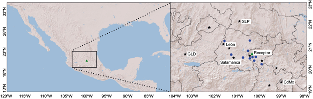
Fig 1 Study region. The green triangle represents the receptor site; black stars represent main urban areas; blue circles represent the climatological stations from the Servicio Meteorológico Nacional (National Weather Service).
The orography of the region is defined by three key features: (1) the Trans-Mexican Volcanic Belt, which runs northwest to southeast, and where the MAQ is located; (2) the Central Mexican Plateau, which lies northwest and west of the MAQ, and (3) the Sierra Madre Oriental, a mountain range running northeast and east of the MAQ, beyond the limits of the Central Plateau. The Sierra Madre Oriental greatly affects precipitation as it forces orographic lifting, promoting rain on the windward side and inhibiting it on its leeward side.
The receptor site for this study was located at the National University Campus Juriquilla (JUR) on the northern border of the MAQ (20° 35’ 35” N, 100° 23’ 32” W, 1945 masl) because it is the host of a monitoring station, part of a University Network of Atmospheric Observatories. The station collects atmospheric data such as meteorology parameters and concentration of criteria pollutants.
2.2 Trajectory calculations
Four years (January 2014 to December 2017) of three-dimensional 12-h back trajectories reaching the JUR site, were calculated using the HYSPLIT model release 4.9 (Draxler and Hess, 1998; HYSPLIT, 2021). Trajectories were calculated at 100 and 500 m above ground level (magl) every 6 h (05:00, 11:00, 17:00, and 23:00 UTC). UTC time corresponds to local time minus 6 h in general, or minus 5 h during daylight saving time. Twelve-hour trajectories were chosen in order to keep the uncertainty results as small as possible, while encompassing important regional sources such as industrial parks and the Salamanca refinery. The HYSPLIT toolbox for Python (PySPLIT, 2021) was used to automatize trajectory generation and analysis (Warner, 2018).
HYSPLIT was driven by the wind fields from the North American Mesoscale (NAM) model, which is maintained by the National Centers for Environmental Prediction (NCEP) of the National Ocean and Atmospheric Agency (NOAA) with a horizontal resolution of 12 km (NAM, 2021).
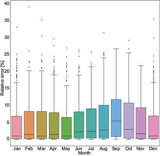
As a control mechanism, a verification process was carried out in order to detect and estimate the HYSPLIT integration error. This process consisted in generating the inverse (forward trajectory) for all the trajectories. A relative error was calculated as the distance between the start of the back trajectory and the end of the forward trajectory, divided by the total distance of both trajectories. Figure S1 in the supplementary material shows the relative errors for all trajectories calculated each month.
Homogenous groups of transport patterns were identified using Ward’s agglomerative hierarchical clustering algorithm, which is included in the HYSPLIT desktop package used to run the model. We looked for the minimum number of clusters that represent all possible flow patterns, using the total spatial variance (TSV) as an aid in this process.
2.3 Surface data
Criteria pollutants (SO2, O3, NO, CO, PM10, and PM2.5) concentration, and surface wind direction and speed data at the JUR monitoring station was obtained from the network website (RUOA, 2021). Wind data goes from June 2014 to December 2017, and pollutants data starts on august in August 2014. CO data ends in November 2017, and NO2 in September 2017.
Additionally, temperature and precipitation data at 11 climatological stations close to the receptor site was obtained from the Servicio Meteorológico Nacional (National Weather Service, SMN) (CONAGUA, 2021). All stations are randomly scattered across the region surrounding the MAQ in the states of Querétaro and Guanajuato (see Table SI and Fig. 1).
3. Results and discussion
3.1 Trajectories
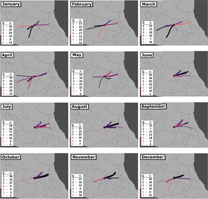
Some files from the NAM database were corrupted or not available for downloading. Therefore, 2% of the trajectories could not be simulated. In addition, trajectory integration errors greater than two standard deviations of the average relative error of the month (approximately 5% of the total) were discarded. All the remaining trajectories (a total of 5490) were grouped by month, independently of the year. Next, the clustering algorithm was applied to obtain the main transport pathways for each month. This procedure was performed separately for both the 100 and 500 magl trajectories, and the results are shown in Figures 2 and S2, respectively. The comparison of both figures shows that flow regimes at both heights are similar; albeit slightly faster at 500 magl, as the wind above is less affected by the surface. The similarity between heights is in agreement with other authors (Eneroth et al., 2003; Markou and Kassomenos, 2010). Because of this, and the fact that emission sources lie on the first 100 m above the surface, we will focus on the results for 100 magl in the rest of the manuscript.
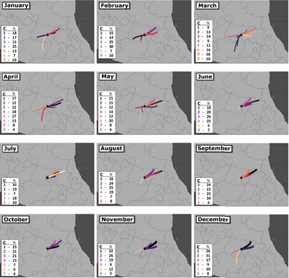
Fig 2 Monthly trajectory clusters calculated for the period 2014-2017, at 100 magl. The thickness of each line is proportional to the percent of trajectories in each cluster, which is specified for each month.
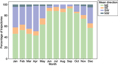
We also calculated the mean direction of all trajectories considering the angle of the vector difference between their endpoint and starting point, and classified them as northeast (NE, 1-90º), southeast (SE, 91-180º), southwest (SW, 181-270º) and northwest (NW, 270-360º). Figure 3 shows the percent of trajectories with a given direction in each month at 100 magl. The figure clearly shows that from June to October, more than 80% of the trajectories originated NE from the MAQ, in contrast to December to April with less than 50% of trajectories with this direction.
3.2 Surface wind and climatology data analysis
Figure 4 shows the monthly frequency of wind direction, as measured at the JUR station from June 2014 until December 2017. In general, winds were observed predominantly from the NE from June to October. However, starting November, northerly winds increased their frequency becoming predominant in January and February. From December until May, strong winds from the southwest were also observed. Wind roses for these months show a wider and more homogenous distribution of wind direction. Previous studies show that wind direction measured at JUR is coherent with wind direction measured in other sites within the MAQ (Camacho-Díaz, 2013; Olivares-Salazar, 2016), which suggests that the transport pathways found in this work might apply to the whole urban area.
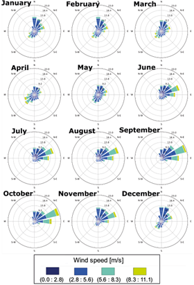
Fig 4 Monthly frequency of wind direction at the RUOA Juriquilla station (receptor site), from June 2014 until December 2017.
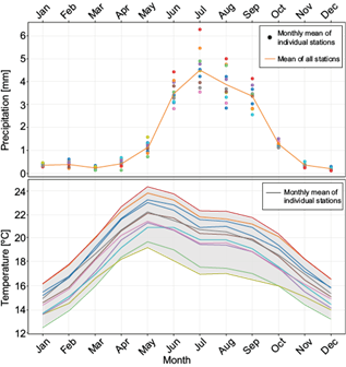
The climatological data of the selected 11 stations in the region is shown in Figure 5. The months with highest precipitation were June to September, with very little precipitation from November to April. Although the variability on precipitation reported among stations increased during the rainy months, the trend was the same for all stations. On the other hand, temperature increased from January until May, when it reached its maximum. After the rainy months began, temperature dropped a couple of degrees and remained relatively constant until October, when it started to drop again, reaching a minimum in December.
3.3 Seasonal transport pathways
The comparison of trajectories direction variability with local and regional wind and rain conditions shows that they all were consistent among two regimes. The temperature did not seem to have a correlation with those regimes.
The rainy regime, from June until September, was characterized by the largest amount of precipitation during the year. In these months, the flow regime was overwhelmingly from the east and northeast, which was clear in both the trajectories (with as few as 5% of the simulated trajectories coming from any other direction) and the wind roses at the receptor sites.
From December to May, very little precipitation was observed, so we defined this period as the dry regime. During these months, the flow regime had an important fraction of trajectories from the NE; however, many were also from the south and west. For March and April, this flow makes up approximately 50% of the total flow. This agrees with wind roses at JUR, which show winds coming from the north and NE, as well as SW
Surface measurements show an important northerly component of the wind for January and February, which is not present in the trajectory results. This situation could be explained by a microscale flow that is not captured by the 12-km NAM model. Other studies which include wind surface measurements at different points at the MAQ do not show this northerly component (Camacho-Díaz, 2013; Olivares-Salazar, 2016), which supports this explanation.
October and November did not exhibit consistent behavior among all the variables being considered; hence, we classified them as “transition months”. For example, October exhibited some rain, and had a wind rose at JUR similar to the one during the rainy regime; but the trajectories from the SW were more frequent, exhibiting a similar pattern to the one seen in November.
Based on this classification, trajectories were grouped by regime and the clustering algorithm was applied again, obtaining the main transport pathways for each regime, shown in Figure 6. This figure constitutes the flow climatology of the MAQ and surrounding region for the period 2014-2017.
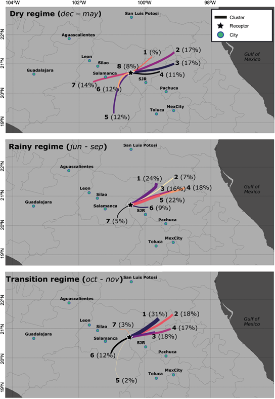
Fig 6 Flow climatology of the MAQ and surrounding region for the period 2014-2017, at 100 magl. The thickness of each line is proportional to the percent of trajectories in each cluster.
In order to validate the proposed flow climatology, we employed the NARR database (Mesinger et al., 2006; NARR, 2021), which uses the high resolution NCEP Eta Model (32 km/45 layers) together with the Regional Data Assimilation System (RDAS) to generate outputs every 3 h. Figure 7 shows wind field data in two different time ranges: 2014-2017, corresponding to the same period as the trajectories calculated in this work; and 1979-2019, corresponding to the climatology of the region. The wind directions observed during 2014-2017 are similar to those during the climatology (1979-2019); however, winds seem to be somewhat weaker during 2014-2017 in December-May and October-November, but stronger in June-September. These results indicate that the years studied in this work were not atypical in comparison with a longer timeframe.
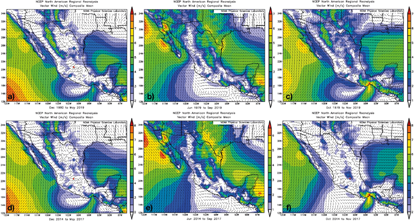
Fig 7 NARR derived wind fields during 1979-2019 (top) and 2014-2017 (bottom) periods, for (a and d) dry regime, (b and e) rainy regime, and (c and f)transition months. The red triangle represents the receptor site (JUR) used in the trajectory analysis.
In the comparison between the trajectories produced and the NARR (2014-2017) (Figs. 6 and 7) there is a coincidence between the direction of the most frequent trajectories and the average wind during the three regimes. During December-May, it is also observed that the receptor site is located in a convergence zone, which is why the dominant components of the trajectories are located in the NE and SW. Finally, it is evident that the trajectories and the winds derived from NARR have shorter paths that follow the surface topography. This is also observed in a closer look at the trajectory’s paths: they never cross the highest topographic features (> 2200 masl) such as the Trans-Mexican Volcanic Belt and the Sierra Madre Oriental.
3.4 Criteria pollutants
Figure 8 shows the monthly mean and standard deviation concentration of SO2, CO, NO, O3, PM10, and PM2.5 at the receptor site during the study period. All these pollutants displayed two maxima in December and April or May, with the exception of O3, which only displayed the April maximum. The lowest concentration of O3 was observed in December; for the rest of the pollutants, the minimum was observed in September.
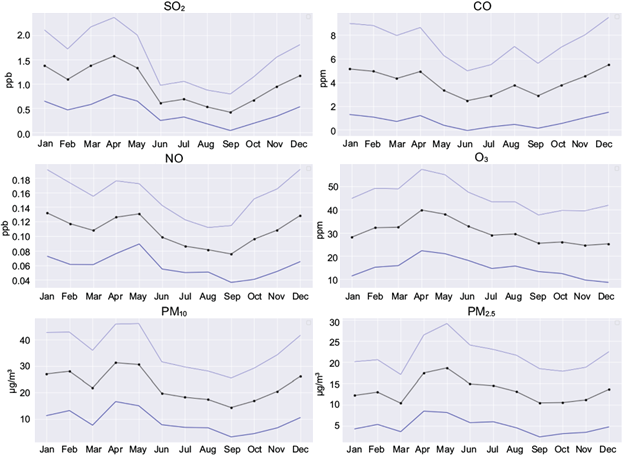
Fig 8 Monthly mean (black dots) of criteria pollutants at the receptor site during the study period. Blue lines represent mean ± standard deviation.
SO2, CO, NO, and PM10 are primary pollutants whose concentrations are strongly related to emissions and transport. The main emission source of SO2 is industry which, for the MAQ, represents a regional source (for example, the industrial corridor León-Irapuato-Salamanca). CO and NO are of industrial origin; however, they are also locally emitted by vehicles. PM10 is mainly regionally emitted by industry, and by resuspension in a semi-arid climate. Hence, it is unsurprising that the highest concentrations of these pollutants were observed during the dry season, when winds from the west were observed. The two maxima observed in the concentrations during this regime were probably related with meteorological factors such as temperature inversions during the coldest months.
In order to explore the relationship between the estimated trajectories, regional emissions, and pollutant concentrations at MAQ, we determined the frequency of the mean direction (see section 3.1) of the trajectories in days with high and low concentrations of SO2 at the receptor site during the dry regime. To do so, we calculated the media (C) and standard deviation (SD) of the daily averages of SO2 concentrations. Days with daily average SO2 > C + 2SD were classified as high SO2 concentration level; days with daily average SO2 < (C - 2SD) were classified as low SO2 concentration level. Figure 9 shows the percent of trajectories with a given mean direction for days with high and low SO2 concentrations at 100 magl during the dry regime. Results indicate that during high SO2 days, 70% of the trajectories originate on the SW direction. In low SO2 days, only 40% of the trajectories originate on this direction and 50% on the NE direction. These results suggest that emissions on the SW quadrant might be affecting the air quality at MAQ.
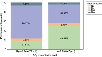
Fig 9 Percent of trajectories with a given mean direction for days with high and low SO2 concentrations, during the dry regime, at 100 magl.
For O3, being a secondary pollutant, its concentration might be more dependent on meteorological conditions that affect reaction rates, such as temperature and radiation, rather than on wind direction. In the beginning of the year, high temperatures and radiation combined with weak winds (Fig. 4) might generate the large O3 concentrations observed. The same is observed in Mexico City, where the O3 season spans from mid-February to mid-June (Zavala et al., 2020). For the MAQ, transport of ozone precursors from the industrial areas during the dry regime, might also contribute to the high concentrations of this gas. During the rainy regime, with no winds from the west, as well as faster local winds and rain, pollutants concentrations decreased.
4. Conclusions
Each cluster in Figure 6 represents a main transport pathway of the flow regime towards the MAQ. The percentage of trajectories assigned to a cluster (and the thickness of the line) indicates the expected frequency of the air following the path of that cluster during that regime. It is evident that a NE flow is present throughout the year. Trajectories from the SW also occur all year long, but they are much less frequent during the rainy regime and the transition months. The clustering algorithm groups trajectories not only by mean direction, but also by longitude and curvature. Hence, short clusters are composed of slow-moving trajectories or trajectories with a high degree of curvature that remain close to the receptor site. The meteorological conditions that give rise to this kind of flow are calm winds or recirculation. The result of both is that air might remain stagnant above the same area facilitating the concentration of pollutants. These clusters are observed during the dry regime and transition months.
It is important to remark that the analyzed period (2014-2017) is consistent with a longer period of time (1979-2019), which implies that the results adequately represent the average conditions of the atmosphere at the study site. Furthermore, the wind patterns of El Bajío are strongly related to the orography of the region.
Some of the trajectories from the NE originate within a desertic region of the state of Querétaro (NE from the MAQ), where several limestone mines are located. Dust resuspension might be common there, especially during the dry months. During the dry regime and transition months, it is clear that some clusters originate in the industrial area of Guanajuato, which includes the Salamanca refinery. Because air transport of pollutants follows these paths, regional sources might be affecting the MAQ air quality.
It is noticeable that no clusters show any transport from the SE of the MAQ, so it is unlikely that there is a contribution of pollutants from Mexico City and its surroundings probably due to the presence of the Trans-Mexican Volcanic Belt south of the MAQ.
This study describes for the first time a flow climatology in central Mexico, which might be useful for finding both geographical and temporal patterns of the wind driven transport of the region. The results raise important questions regarding regional sources of pollutants that might be affecting the air quality. Future studies should address the influence that industrial areas around the MAQ, in El Bajío, have on the concentration of air pollutants such as ozone and particulate matter. They should also weigh the effect of local emissions, regional transport, and meteorological conditions on the air quality of the region.