nueva página del texto (beta)
 Inglés (pdf)
 Artículo en XML
 Referencias del artículo
 Enviar artículo por email
 Citado por SciELO
  Similares en
SciELO
Similares en
SciELO 
 Permalink
1. Introduction
Ground-level ozone (O3) is a secondary air pollutant formed in the troposphere via the photo-oxidation of carbon monoxide (CO), methane (CH4), and volatile organic compounds (VOCs) in the presence of nitrogen oxides (NO+NO2 = NOX) (Jenkin and Clemitshaw, 2000). It is of concern to policymakers due to its adverse impacts on human health, agricultural crops, and vegetation (Lefohn et al., 2017). The occurrence of higher concentrations of ground-level O3 during weekends than on weekdays in urban areas is known as the “O3 weekend effect” (OWE) and arises from changes in anthropogenic activity from weekdays-to-weekends (Heuss et al., 2003). The system of O3 production is not linear which may lead to similar or significantly different O3 concentrations between weekdays and weekends (Monks et al., 2015; Heuss et al., 2003). The OWE occurrence in urban areas has been studied extensively in the West Coast, Midwest and East Coast of the US (Marr and Harley, 2002; Heuss et al., 2003; Atkinson-Palombo et al., 2006; Baidar et al., 2015; Blanchard et al., 2008; Wolff et al., 2013), as well as in several other major cities around the world (Rozbicka and Rozbicki, 2016; Zhao et al., 2019; Sadanaga et al., 2012; Seguel et al., 2012; Zou et al., 2019).
In order to assess the temporal changes in OWE occurrence, several approaches have been used including i) statistical analysis of monitoring data for ambient O3 (Blanchard et al., 2008; Wolff et al., 2013), ii) photochemical modelling (Yarwood et al., 2003, 2008), iii) intensive field campaigns (Fujita et al., 2002), and iv) analysis of measurements of the O3 vertical column density (Baidar et al., 2015). Overall, there is agreement that the OWE is caused by larger reductions during weekends in emissions of NOX than in VOCs, driven mostly by changes in the vehicular activity in VOC-limited conditions (Heuss et al., 2003; Blanchard et al., 2008). Those large reductions in NOX emissions increase the VOC/ NOX ambient ratio, enhancing O3 production and simultaneously reducing O3 titration (Fujita et al., 2002; Marr and Harley, 2002).
While most existing studies have focused on quantifying the temporal changes in OWE, its spatial evolution has received less consideration. The OWE spatial occurrence may vary from city-to-city and within cities, but its understanding and quantification can provide valuable insights into the design of potential air quality control strategies. To address spatial variations in air pollutants, the network analysis approach has been used previously to i) identify clusters among monitoring sites in China using ground-level data for fine particulate matter (PM2.5) (Yan and Wu, 2016) and ii) to represent interactions in PM2.5 levels between cities, also in China, using motifs and weighted networks (Wang et al., 2017, 2018). This suggests that a network can be used also for representing the OWE spatial interaction and its evolution in order to provide an approximation of its spatial spread within urban areas. Indeed, the network construction requires few variables in comparison with those typically used in photochemical modelling (Garcia-Reynoso et al., 2009; Kanda et al., 2016), representing an advantage for cities with limited monitoring and modelling resources.
Analysis of the predictability of the OWE may provide information on the existence of temporal patterns and other correlated variables beyond the commonly used linear regression in O3 data. This analysis measures the ability of univariate models such as ARIMA, Linear and Naïve, to generalise the O3 behaviour by minimising forecast errors. Therefore, the detection of patterns in OWE using recorded data for O3 is a practical way to anticipate, with certain accuracy, future magnitudes of the OWE. Although the prediction approach has been used previously by Jiménez et al. (2005) and Garcia-Reynoso et al. (2009), these studies focused on finding the origin for high O3 concentrations during weekends rather than in minimising and validating the OWE prediction. Additionally, Baidar et al. (2015) modelled the OWE as a non-parametric probability distribution function to identify how the probability of occurrence of the OWE has changed in California, USA between 2003 and 2014. Although, this approach could be used to predict the OWE as a random variable, it is limited in representing more complex temporal variations.
As in other metropolitan areas, the few existing studies for OWE within the Mexico City Metropolitan Area (MCMA) have focused on understanding its origin and long-term trend. Overall, ground-level O3 within the MCMA decreased over the past three decades following controls that targeted at industrial and mobile precursor emission sources (Rodriguez et al., 2016; Hernández-Paniagua et al., 2017; Velasco and Retama, 2017; Ramos-Ibarra et al., 2020). However, the declining rate of O3 has slowed down since 2013 and in 2015 reached a stationary state, which has subsequently resulted in the occurrence of episodes of significantly high O3 concentrations recurrently since 2016. Moreover, Stephens et al. (2008) reported no significant differences in O3 concentrations between weekdays and weekends during 1986-2008, which contrasts with the report of Hernández-Paniagua et al. (2018) who observed, on average, higher O3 peaks on weekends at some monitoring sites over 1988-2016. This highlights the importance of obtaining precise information about spatio-temporal past and future changes in OWE occurrences in an effort to control ground-level O3.
We present here a spatio-temporal assessment of the OWE occurrence within the MCMA using 1-h O3 data recorded during 1994-2018 at ten monitoring sites distributed among different land use categories, traffic flows and spatial locations. Metrics reported in the literature calculated from daily O3 peaks between weekends and weekdays are used to detect the OWE occurrence and magnitude at each site. Long-term trends in the OWE occurrence and magnitude are quantified using the non-parametric Theil-Sen method and ARIMA models. To account for the OWE spatial variations, annual networks are built with nodes representing monitoring sites and edges corresponding to similarity between OWE magnitudes.
We also propose the definition of generalised OWE (GOWE), which allows the identification of year-to-year changes in OWE occurrences represented by a sequence of graphs (networks). Finally, common measures are calculated for graphs representing the GOWE which permit the detection of spatial patterns with respect to changes in the OWE. To our knowledge, this is the first study that has considered the use of networks for analysing and predicting spatial interactions in the OWE occurrence. Therefore, we discuss how the proposed approach can be used to identify clusters or groups of monitoring sites with similar OWE magnitudes and to predict changes in the OWE in a city or geographical area.
This paper is organised as follows: Section 2 presents the metrics and formal definitions used to calculate long-term trends in OWE and build networks. Section 3 presents the data quality and methods used to calculate the temporal trends and structures presented and the network measures used to quantify spatial interactions among monitoring sites. Section 4 describes in detail the OWE occurrence and its spatio-temporal evolution within the MCMA. Finally, Section 5 provides conclusions regarding the methods implemented here to quantify spatio-temporal trends in OWE and from the results obtained.
2. Network representation of the OWE
2.1 OWE metrics definition
The network representation of the OWE is introduced to analyse the spatial interaction among monitoring sites when it is detected within a city or geographic region. In order to simplify the notation, each monitoring site (s) is represented here as a natural number
The OWE occurrence has been calculated in existing studies using three main statistics (Atkinson-Palombo et al., 2006; Blanchard et al., 2008; Garcia-Reynoso et al., 2009), which are detailed as follows:
Differences in 1-h maximum concentrations between Sunday and Wednesday within the same week, denoted as OW1s = max(u s sun) - max (u s wed).
Differences in 1-h maximum concentrations between Saturday and Wednesday within the same week, denoted as OW2s = max(u s sat) - max (u s wed).
Differences in daytime (06:00-18:00 CDT) O3 averages (avg) between weekend (Saturday-Sunday) and weekdays (Tuesday-Wednesday-Thursday), denoted as OW3s = avg(w s sat,u s sun) - avg(w s tue, w s wed, w s thu). In each case, the average is calculated for the concatenation of the corresponding vectors.
Monday and Friday are considered as transition days in the MCMA and were not included in the calculation of the weekday averages because these are influenced by the carryover from the previous days (Atkinson-Palombo et al., 2006; SEDEMA, 2018). In general, the notation OW s is used to refer to any of the three measures presented above, i.e. OW s can refer to OW1s, OW2s or OW3s. In this way, when OW s > 0 there is OWE occurrence in monitoring site s; otherwise, there is no OWE occurrence. In addition, when it is not necessary to refer to a particular monitoring site, OW1, OW2, OW3 and OW are used. Among the three metrics considered, OW3s may capture the effect of high ground-level O3 concentrations and the periods that these last, while OW1s and OW2s describe the occurrence of high O3 concentrations without considering their duration. Nevertheless, since our approach is devoted to describe spatio-temporal interactions in the OWE rather that its duration, any metric can be used.
2.2 Spatial networks of the generalised OWE
The OWE spatial intensity and spread within an urban area or region can be approximated using the concept of GOWE and represented as a network, as described in Definition 1.
Definition 1. Given a geographic region C and a set S of monitoring sites localised in C, there is GOWE occurrence during a given weekend if at least half of the monitoring sites exhibit OWE occurrence.
If the OWE spatial intensity in C is represented by the number of monitoring sites with OWE occurrence, then it can be stated that the GOWE reveals high spatial intensity. Additionally, in order to approximate the OWE spread, the graph (network) is used to represent the GOWE in which the vertices (nodes) are the monitoring sites and the edges (links) represent similarities in OWE magnitudes.
Let
Definition 2. The OWE is generalised for annual averages (⟨GOWE⟩) if p + ≥ n / 2.
We denote by v y + the vector whose ith component is avg(OW i y) if avg(OW i y) ≥ 0, and 0 otherwise. The network representation of each ⟨GOWE⟩ is built using the Euclidean distance matrix M y for the vector components v y +. The i, j entry of M y is the difference in OWE annual averages between monitoring sites i and j that exhibited OWE in the year y.
Definition 3. Given a set of monitoring sites S and the Euclidean distance matrix M y , the spatial network of ⟨GOWE⟩ in the year y is the graph G(S)y =(V, E) such that V represents the set S and E = {(i, j)|(M y )i,j ≤ avg(vy +)}. Therefore, the existence of an edge between the monitoring sites i and j in G(S)y represents the occurrence of OWE with similar magnitudes between them in the year y.
3. Materials and methods
3.1 Air quality data
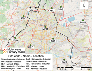
Continuous monitoring of ground-level O3, CO, SO2, NO2, PM10 and PM2.5 have been carried out within the MCMA since 1986, along with seven meteorological parameters (temperature, rainfall, solar radiation, wind speed, wind direction, pressure and relative humidity). O3 is measured with photometric analysers model 49-X UV (Thermo Environmental Instruments Inc.) in accordance with EPA EQOA-0880-047. Calibration, maintenance procedures and data quality assurance/quality control (QA/QC) followed protocols established in the Mexican standards NOM-036-SEMARNAT-1993 and NOM-156-SEMARNAT-2012 (SEDEMA, 2020a). Publicly available 1-h data validated by the Sub-Division of Analysis and Modelling of the Secretariat for the Environment of the Mexico City were downloaded from the SIMAT website (http://www.aire.cdmx.gob.mx; SEDEMA, 2020a). A data capture threshold of 75 % hourly O3 data per day was established to select the monitoring sites with the longest records to study the OWE evolution (Figure 1) (SEDEMA, 2020b).
3.2 Trend analyses
The SIMAT data set was analysed using the openair package v2.6-5 (Carslaw, 2019) and the R software (R Core Team, 2018). All statistical analyses were performed with the R base software. Long-term trends were computed with openair for the R using annual values for occurrences and magnitudes as follows. Firstly, the presence of a monotonic trend was tested with the non-parametric Mann-Kendall test, where the null hypothesis H 0 of no trend is tested against the alternative hypothesis H 1 of some trend. As reported by Carslaw and Ropkins (2012), the H 0 is rejected if the p - value < 0.1. Secondly, slopes of linear trends were calculated with the non-parametric Sen’s method, which assumes linear trends, with an m slope and a b intercept. To calculate m, first the slopes of all data values were calculated in pairs, with the Sen’s estimator slope as the median of all calculated slopes (Theil, 1950). Finally, 95 % two-sided confidence intervals about the slope estimate were obtained based on a normal distribution.
For the trends in OWE occurrences, sensitivity analyses were performed for the number of annual occurrences considering a threshold of 3 ± 1 ppb, following the methodology reported by Baidar et al. (2015). Then, the trends for each threshold were contrasted. For the OWE magnitude trends, annual OWE average magnitudes of each OW were used in order to capture the week-to-week variation.
3.3 Prediction of OW
We provide an analysis that identifies suitable predictive models for each OW time series from the univariate perspective. These simple statistical time series models allow the generation of a prediction of an OW network with a given level of uncertainty. In order to identify a prediction model for OW, a set of simple models are fitted at each time series sample, which are listed below:
Autoregressive Integrated Moving Average (ARIMA, ARMA) Models.
A linear regression model vˆy +1 = my + b estimated with Theil-Sen Slopes.
A Naive model (vˆy +1 = = v y) that uses the last observed OW as the prediction.
Briefly, an ARIMA model is a composition of two statistical models for stationary time series: an Autoregressive (AR) and a Moving Average (MA) components of order P and Q, respectively (Montgomery et al., 2011). Each order defines the number of coeffifcients applied for each model. The integrated part is represented with D ≥ 0 and describes the number of times that the time series needed a differentiation transformation to make it stationary (D = 1 means the computing of the first time series differences).
In order to conduct the predictability analysis using cross validation, the v (OW) times series was organised in: i) training, ii) test and iii) validation sets. With the training set, an ARIMA or ARMA structure was identified using the auto.arima function included in the forecast package version 8.1 (Hyndman et al., 2020) for R software. The auto.arima function in R implements by default the Hyndman-Khandakar algorithm which consists of the following steps. Firstly, it finds the number of differentiation processes (D) required to remove the trend if exists using the Kwiatkowski-Phillips-Schmidt-Shin test (KPSS) (Kwiatkowski et al., 1992). Once D is obtained, a set of ARIMA models in a bounded model space defined by the maximum P and Q order is optimised using the conditional-sum-of-squares for estimating initial coefficient values. Then, to improve the model fitting maximum likelihood is used (R Core Team, 2018). Finally, the model selected is the one with the minimum Akaike Information Criterion (AIC) value (Hyndman and Khandakar, 2008).
Similarly, the linear regression was calculated for the training set used with ARIMA, using the Theil-Sen method implemented in SciPy (Virtanen et al., 2020). For the Naive model, no training step was required. Each model performance was evaluated by analysing the residuals obtained. The probability of rejecting the hypothesis of null autocorrelations H 0 at lags 1 to 4 of residuals was tested using the Ljung-Box test (Greene, 2003). If the test fails, the model is probably biased or not significantly capturing the correlations presented in the time series (H 1 ), otherwise, the residuals approximate a normal distribution with mean centred in 0 with no temporal autocorrelations (H 0 ), suggesting the suitability of the model. Such property can be confirmed or rejected depending on data availability. This test was complemented with the prediction performance describing how similar are the OW predictions to real OW data considering the Mean Absolute Errors (MAE) of residuals, defined as 1/N ∑N y=1 | r y ts |, where N is the OW set size and r y ts = v y ts - vˆy ts are the residuals from the test set. The model with the minimum MAE and significant statistical fitting (no residual autocorrelations) was selected as the best predictor, and its accuracy was validated with the last OW value available at each monitoring site.
In order to select the best model in the scenario when two models present similar performance, we performed a Student’s t-test (Student, 1908) of independent means with unknown variance using SciPy, where the means are computed from the residuals of the two best models in order to detect high probability of statistically similar performances. This test is valid when discarding models producing residuals with possible non-normal distribution. Otherwise, other kind of independent means test could be considered such as the Diebold-Mariano (Diebold and Mariano, 2002).
3.4 Network measures
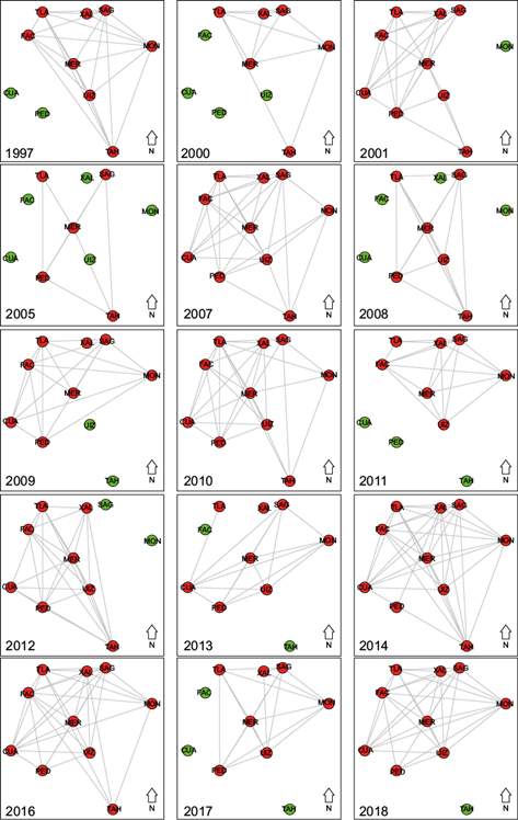
Following Definition 3, a sequence of graphs G = G(S)1,…, G(S)κ was built, where κ equals to the number of years with ⟨GOWE⟩. Figure 2 shows the graph for the MCMA using the vector v 4 with the measure OW1 for 2005. In that network, only five monitoring sites exhibited OWE annual occurrence. It should be noted that in Figure 2a the network shows geographical reference, while Figure 2b does not include it, which is useful to better show all connections among monitoring sites.
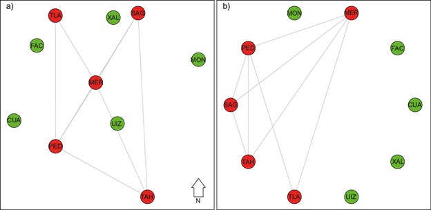
Fig. 2 Spatial network for ⟨GOWE⟩ within the MCMA in 2005. The vertices represent the monitoring sites spatial location within the MCMA. The green vertices show monitoring sites with no average OWE annual occurrence, whereas the red vertices show monitoring sites with average OWE annual occurrence. a) The ⟨GOWE⟩ network with geographical reference of monitoring sites. b) The same ⟨GOWE⟩ network but without geographical reference.
In order to characterise the networks’ structure and connectivity, the following measures were calculated: clustering coefficient, average path length, the size of the largest clique and the algebraic connectivity of each graph in G (Newman, 2003). These measures are relevant because they allow to find groups of nodes that share attributes, such as the number of connections among nodes and strength of these connections. For instance, the size of largest cliques of nodes can be used as a proxy of the OWE magnitude within urban areas, i.e. the larger the size of the clique the greater the similarities in OWE magnitudes. Additionally, the average path length and transitivity are useful to identify the small world property, in the context of OWE, a network with this property could imply large spatial spread of the OWE within the city. The mathematical description of these measures is given below:
The clustering coefficient or transitivity defined as C = 3τΔ/τ3, where τΔ equals to the number of triangles in the graph and τ3 is the number of connected triples. In the case of network in Figure 2, its transitivity is 0.789 because almost all possible triangles are present given the connected triples.
The average path length of each graph is ⟨l⟩ = 2/n(n - 1) ∑n i,j=1/i≠1 l ij , where n is the number of vertices in the graph and l ij is the distance between vertices i and j, we recall that this distance is defined as the length of the shortest path between such vertices. The ⟨l⟩ of the network in Figure 2 is 1.2, meaning that in average, every node is connected with other node in one step.
The size of the largest clique (lc) in the network is defined as the largest complete subgraph, meaning that each vertex is connected to all vertices in the graph. In the case of the network in Figure 2, the lc is equal to 4 and the clique is the subgraph with vertices MER, PED, SAG and TAH. This means that there is a strong relation among them with the rest of vertices.
The second smallest eigenvalue (λ 2 , also called the algebraic connectivity) of the graph Laplacian, which is defined as the matrix L = D - A, where A is the adjacency matrix of the graph and D is a diagonal matrix with D ii = d i , where d i is the degree of vertex i. The λ 2 of network in Figure 2 is 2, we recall that the maximum value of λ 2 equals to the number of vertices in the graph, hence a value of 2 suggest a weak connection. It should be noted that λ 2 is very sensitive to pendant nodes but it is incorporated as a benchmark of the networks connectivity.
The significance of those measurements was tested by comparing their empirical distributions against distributions of random graphs (Milo et al., 2002). We built random graphs using the Erdös-Renyi model G(n, m) (Kolaczyk and Csárdi, 2014). All network calculations were made using the igraph package (Csardi and Nepusz, 2006) in R software.
4. Results and discussion
The present section is organised as follows. Firstly, the OWE annual occurrence is described for each monitoring site. Secondly, long-term trends in OWE annual occurrences and magnitudes are presented for those sites that showed statistically significant changes. Finally, the metrics that exhibited significant trends are used to evaluate the OWE spatial spread and to predict its annual occurrence.
4.1 The OWE annual occurrence
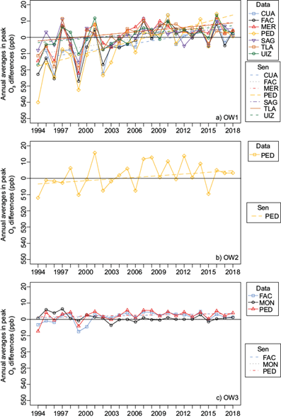
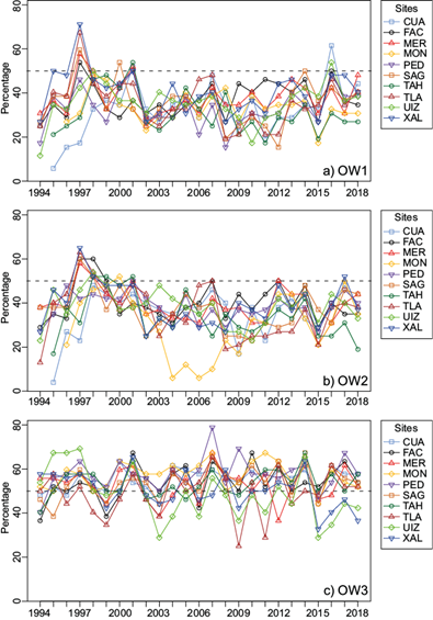
In order to calculate long-term changes in the annual percentage of OWE occurrences within the MCMA during 1994-2018, the OW1,OW2 and OW3 metrics were analysed. The annual percentage of OWE occurrences at a given monitoring site is calculated from the number of weeks that showed OWE occurrence in a calendar year. The OWE annual occurrence for OW2 and OW1 ranged between 4-65 % and 6-71 %, respectively, and between 25-79 % for OW3, with most of the annual occurrences ranging between 20-50 % for OW1, OW2, and between 40-65 % for OW3. Uncertainty in the annual percentage of OWE occurrences was calculated as the counting error ( /(2N)) (Baidar et al., 2015), where N is the number of weeks that contain measurements to calculate OW1, OW2 and OW3. The uncertainty in OWE annual occurrences for all years and all metrics was lower than 1 %. Annual OWE occurrences were used to test the presence of long-term trends. Overall, no significant trends (p > 0.1) were observed for OW1 and OW2 despite periods of apparent increases (1994-1998) and decreases (1998-2003), observed at most of the monitoring sites (Figure 3a,b). By contrast, OW3 showed significant increasing trends (p < 0.1) of similar values at the downwind sites of PED (0.81 % yr-1) and FAC (0.89 % yr-1), while significant decreases were detected at the peri-urban MON (-1.35 % yr-1) and TAH sites (-0.97 % yr-1) (Figure 3c).
4.2 The increasing magnitude in OW
Figure 4 shows the sites that exhibited significant trends in the OWE annual magnitude within the MCMA and Table I summarises the parameterisation of the trends. Overall, during 1994-2018 in the MCMA, the three metrics showed significant trends (p < 0.1) in at least one monitoring site, mostly at downwind sites. For instance, OW2 showed an increase (p < 0.05) only at PED of 0.51 ppb yr-1, while OW1 showed increases (p < 0.1) at seven monitoring sites ranging from 0.33 ppb yr-1 at UIZ to 1.31 ppb yr-1 at PED. The lowest growth rates (p < 0.1) were observed for OW3 and ranged from 0.10 ppb yr-1 at FAC to 0.18 ppb yr-1 at PED. It is worth noting that only the downwind PED site exhibited significant increasing trends for all metrics and also showed the largest increases among all sites. This indicates a combination of higher net O3 production derived from the occurrence of photochemical processed air masses and low titration rates due to reduced NOX emissions at upwind and core regions (Table I) (Jaimes-Palomera et al., 2016; SEDEMA, 2018). By contrast, among the sites that exhibited significant changes, only MON, which is a peri-urban and upwind site, exhibited a significant decreasing trend (p < 0.05) in OW3 of 0.1 ppb yr-1. This can be explained as MON is less affected by changes in precursor emissions from the urban area.
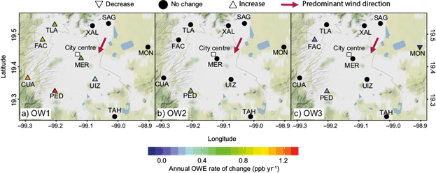
Fig. 4 Annual growth rates in the OWE magnitudes within the MCMA during 1994-2018 by metric. Sites with no significant trends (p > 0.1) are represented by black-filled circles.
Table I Results for OWE long-term trends by metric during 1994-2018 within the MCMA with slopes expressed in ppb yr-1.
| Site | OW2 | OW1 | OW3 | ||||
| ppb yr-1 | Sig. | ppb yr-1 | Sig. | ppb yr-1 | Sig. | ||
| CUA | 0.20 [-0.23, 0.64] | 1.14 [0.74, 1.46] | * | 0.06 [-0.10, 0.27] | |||
| FAC | 0.23 [-0.40, 0.82] | 0.82 [0.06, 1.43] | * | 0.10 [-0.03, 0.23] | + | ||
| MER | 0 [-0.32, 0.50] | 0.48 [-0.03, 0.99] | + | 0.03 [-0.09, 0.18] | |||
| MON | 0.03 [-0.50, 0.38] | 0.25 [-0.11, 0.53] | -0.10 [-0.14, 0.05] | * | |||
| PED | 0.51 [0.02, 0.72] | * | 1.31 [0.63, 1.95] | *** | 0.18 [-0.04 , 0.39] | * | |
| SAG | 0.13 [-0.41, 0.37] | 0.53 [0.16, 0.88] | 0.04 [-0.06 , 0.13] | ||||
| TAH | 0.11 [-0.36, 0.17] | 0.17 [-0.13, 0.42] | -0.03 [-0.13, 0.05] | ||||
| TLA | 0.05 [-0.31, 0.30] | 0.51 [-0.03, 0.97] | * | -0.03 [-0.13, 0.05] | |||
| UIZ | -0.09 [-0.44, 0.36] | 0.33 [0.03, 0.92] | * | 0.03 [-0.09, 0.13] | |||
| XAL | 0.06 [-0.29, 0.44] | 0.13 [-0.26, 0.82] | -0.02 [-0.14, 0.13] | ||||
The numbers show the trend estimate together with the lower and upper 95 % confidence intervals in the slope shown in brackets. Note also that the significance (sig.) column shown relate to how statistically significant the trend estimate is: +Level of significance p < 0.1. *Level of significance p < 0.05. **Level of significance p < 0.01. ***Level of significance p < 0.001. The absence of a symbol means that there is no statistically significant slope detected.
The largest OWE magnitude changes are detected for OW1, which suggests that only Sundays present significant reductions in NOX emissions due to net reduced vehicular activity. This is consistent with the study of Davis (2017) who reported no significant changes on pollutants levels on Saturdays in the MCMA, including CO and NOX which are mostly emitted by vehicles, despite the introduction in 2008 of license-plate based driving restrictions. Therefore, it is likely that the existence of non-apparent trends in OW2 is due to non-significant reductions in vehicular activity on Saturdays. Furthermore, the OW3 metric did not exhibit increasing trends at those same sites where OW1 did exhibit trends. This result, arises from averaging Saturday and Sunday O3 data. Our results suggest that OW1 captures more accurately the temporal changes in OWE magnitudes than OW2 and OW3 within the MCMA.
4.3 Prediction of OW
Among the three metrics addressed, only OW1 exhibited significant increasing trends for the OWE annual occurrence at most of the monitoring sites, therefore, OW1 was used to test whether the OWE annual occurrence can be statistically predicted. Each OW1s time series data sequence is divided as follows: the first 60 % of the data correspond to the training set, the next 36 % is used as a testing set and the remaining data (4 %) are used for validation. Table II shows the statistical fitting results and Figure 5 the performance of the models considered here to fit the OW1s time series auto-correlations. In Table II, in the results for the Ljung-Box test 1 (TRUE) indicates that the null hypothesis H 0 cannot be rejected (p > 0.05), while 0 (FALSE) represents the existence of significant auto-correlations between lags resulting in the rejection of the null hypothesis.
Table II Results of the fitting tests applied to the OW1s annual magnitude time series.
| Site | ARIMA (P,D,Q) | Best model | Ljung-Box test for r lags from 1 to 4 | ||
| ARIMA | LINE | Naive | |||
| CUA | (2, 1, 0) | ARIMA | [1, 1, 1, 1] | [1, 1, 1, 1] | [0, 1, 1, 1] |
| FAC | (0, 0, 0) | Line | [1, 1, 1, 1] | [1, 1, 1, 1] | [0, 0, 0, 0] |
| MER | (0, 1, 0) | Naive | [1, 1, 1, 1] | [1, 1, 1, 1] | [1, 1, 1, 1] |
| MON | (0, 0, 0) | Mean | [1, 1, 1, 1] | [1, 1, 1, 1] | [1, 1, 1, 1] |
| PED | (0, 1, 0) | Line | [0, 0, 0, 0] | [1, 1, 1, 1] | [0, 0, 0, 0] |
| SAG | (0, 0, 0) | Line | [1, 1, 1, 1] | [1, 1, 1, 1] | [0, 1, 1, 1] |
| TAH | (0, 0, 1) | ARIMA | [1, 1, 1, 1] | [1, 1, 1, 1] | [1, 1, 1, 1] |
| TLA | (0, 0, 0) | Naive | [1, 1, 1, 1] | [0, 0, 1, 1] | [1, 1, 1, 1] |
| UIZ | (0, 0, 0) | Mean | [1, 1, 1, 1] | [1, 1, 1, 1] | [0, 0, 0, 0] |
| XAL | (0, 0, 0) | Mean | [1, 1, 1, 1] | [1, 1, 1, 1] | [1, 1, 1, 1] |
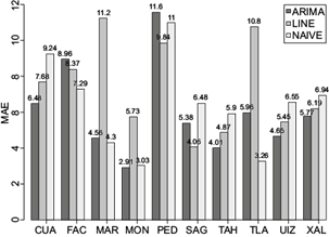
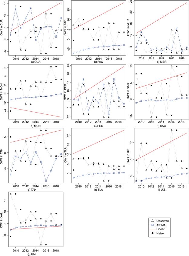
At all sites, the model with the best performance also showed good statistical fitting considering the first lag, i.e. it passed the Ljung-Box test, apart from FAC where Naive showed the best MAE performance (Figure 5) but low statistical fitting (Table II). It suggests that for FAC the existence of good predictions may arise from predicting artefacts due to a change in the OWE temporal dynamic not observed in the training set. By contrast, for CUA and TAH, the ARIMA model that passed the Ljung-Box test showed also the best performance. Similarly, for MON and PED, the linear regression showed the best performance and significant statistical fitting. Our results show that statistical tests permit the determination of the model that best generalises the temporal dynamics of the OW1s time series and predicting the OWE annual occurrence with a given level of confidence. On average, the highest MAEs in OW1s are observed for downwind sites, which can be more influenced in the short-term by large changes in meteorology and in local emissions of O3 precursors and titration. Markedly, the peri-urban and upwind site MON that showed the lowest MAE is less influenced by these changes, particularly in emissions from the whole urban area.
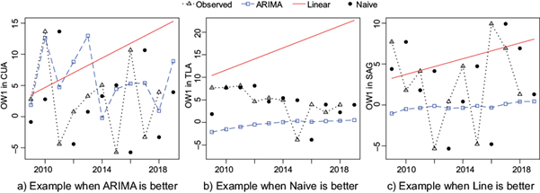
Figure 6 shows a 3-case comparison when the OW1s time series are best fitted by a specific prediction model. The prediction models were selected following the criteria described in Section 3.3, using the results from the Ljung-Box test (Table II), MAE performance and the t-test (Table B.3-4). Figure 6a shows a case when ARIMA and Line better generalise the testing set in CUA; i.e. passed the Ljung-Box test, their means are statistically similar but ARIMA has the minimum MAE, therefore ARIMA was chosen. Figure 6b shows the prediction in TLA when the Naive and ARIMA models pass the Ljung-Box test, but Naive generates the best MAE performance and its residual distribution is statistically different from the ARIMA model leading to select the Naive model. Figure 6c presents the prediction case for SAG where the Linear and ARIMA models both passed the Ljung-Box, but the Line model presents the minimum MAE suggesting closer predictions to the observations and its residuals are statistically different from ARIMA. Therefore, we selected the Line model to fit the data in SAG. After the models’ validation, predictions for the OWE annual magnitudes at all sites were made for 2018 and 2019 (Table II). Those predictions were used in the spatial analysis to compare the results from our predictability approach with the observed data.
4.4 OW spatial and network analysis
Figure 7 shows the relative frequency of the ⟨GOWE⟩ using the different OW s metrics by periods of 5 years. It is clear that the relative occurrence of OW1 increased from 1994 to 2018, resulting in more monitoring sites exhibiting more average OWE occurrences in recent years. By contrast, the relative frequency of ⟨GOWE⟩ for OW2 and OW3 shows less pronounced variations which is consistent with the results obtained in the OWE occurrence and trend analyses. Therefore, only the networks for ⟨GOWE⟩ occurrence for OW1 were analysed and are shown in Appendix E (Fig. E13).
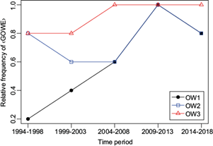
Fig. 7 Relative frequency of ⟨GOWE⟩ occurrences within the MCMA during 1994-2018 by periods of 5 years.
The observed increase in ⟨GOWE⟩ occurrence can be interpreted as the spread of VOC-limited conditions within the MCMA, which arises from more sites exhibit recurrently annual OWE in recent years. This is supported by the observational study of Marr and Harley (2002) who reported that only VOC-sensitive urban areas in California showed significant increases in O3 levels during weekends. In an earlier study in the MCMA, Stephens et al. (2008) reported no significant differences in O3 from weekdays to weekends at most of the monitoring sites between 1986-2007, while Kanda et al. (2016) determined for a period of 2012 that O3 production lies in the VOC-sensitive regime. These separate studies support our hypothesis that VOC-limited conditions are increasing and spreading in the MCMA.
Remarkably, the graphs that correspond to ⟨GOWE⟩ occurrence exhibited the so-called small world effect in all years. Briefly, a small world network is a graph with high C and low ⟨l⟩ (Watts and Strogatz, 1998). Here, transitivity was used instead of the average clustering coefficient that is used in the original model of Watts and Strogatz (1998), because the transitivity can reflect better the global clustering (Estrada, 2016). Figure 8a shows the existence of an inverse relationship between transitivity and mean distance for ⟨GOWE⟩ graphs. However, no significant differences (p > 0.05) were observed when transitivity or average clustering coefficient were used. The small-world property implies that in all graphs, the OWE, and therefore VOC-limited conditions, can spread easily within the MCMA because the average path length is less than 1.5 and may have the same magnitude since the transitivity is at least 0.75. Furthermore, this is observed clearly since 2011 when the annual OWE magnitudes at the sites exhibiting increasing trends vary on average within a range of 10 ppb of difference (Fig. A11a).
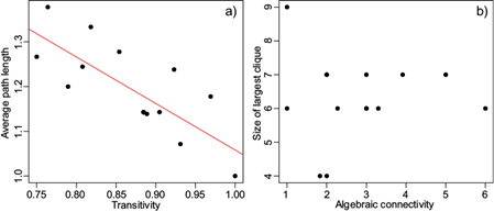
Fig. 8 Comparison of measures for ⟨GOWE⟩ graphs. Scatter plots for a) Average path length and transitivity and, b) largest clique and algebraic connectivity in each graph.
It should be noted that the small-world property does not imply that all graphs have the same kind of connectivity, therefore, the size of the largest clique (lc) and the algebraic connectivity (λ 2 ) were used to characterise the connectivity within the graphs. Figure 8b shows the comparison between λ 2 and lc in each graph. We recall that the algebraic connectivity depends on the number of vertices as well as the kind of connection between them. For the graphs of ⟨GOWE⟩ occurrences, the average lc was 6.2 and ranged between 6 and 7, implying that not only the ⟨GOWE⟩ was comprised by at least five monitoring sites, but also that the OWE annual magnitudes were similar among sites.
Figure 8 shows that the network with the highest value of lc exhibits the lowest value of λ 2 , whereas networks with different values of λ 2 showed the same value of lc. This is explained because λ 2 is highly sensitive to pendant nodes. For instance, the network for ⟨GOWE⟩ for 2014 with λ 2 = 1 and lc = 9 has a pendant node (Fig. E13), meaning that its degree equals to 1 and is similar to that for 2013 with λ 2 = 1 and lc = 6. By contrast, the network for 2008 with λ 2 = 6 and lc = 6 has a complete subgraph with six nodes and implies clearly that these six monitoring sites exhibited OWE with the same magnitude.
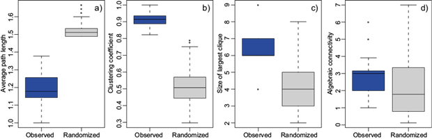
In order to assess the significance of measurements in the ⟨GOWE⟩ graphs, 1000 random networks were built using the Erdös-Renyi model (G(n, m)) with 10 vertices and edges from 8 to 37 edges, similarly to the graphs obtained from observations. Significant differences (p > 0.05) were observed between the measurements for the observed and random networks (Figure 9), whereas only the algebraic connectivity did not show significant differences. Furthermore, the Kolmogorov-Smirnov test was used to test the null hypothesis that the two samples were drawn from the same distribution with a significance level of 0.05 (Marsaglia et al., 2003). A statistic value of 0.375 and a p - value = 0.029 were determined, which allowed the rejection of the null hypothesis. This allows to conclude that the algebraic connectivity distributions were statistically different and the measures calculated to characterise the ⟨GOWE⟩ networks are statistically significant and capture well these OWE structural properties.
4.5 The predicted GOWE occurrence
The univariate OW1 predictions presented in Appendix D are used to represent an approximation of the ⟨GOWE⟩ occurrence for the MCMA. Two networks of ⟨GOWE⟩ were built for 2018 and 2019 using the predicted data for OW1, and Figure 10 shows the comparison between networks built with observed and predicted data. The predicted data suggest a ⟨GOWE⟩ occurrence in 2018 in good agreement with the observed data and those predicted also suggest ⟨GOWE⟩ occurrence for 2019. Additionally, for 2018 and 2019, the ⟨l⟩s and Cs values for the forecasted networks were 1 (complete networks), in good agreement with the range of values determined for the observed networks. Our results were accurate in predicting OWE occurrence for TLA and MER in 2018 as observed in the graphs built from observed data when there is ⟨GOWE⟩ occurrence. According to our results obtained from the prediction approach, the ⟨GOWE⟩ will continue occurring within the MCMA and is likely to comprise more monitoring sites in future years.
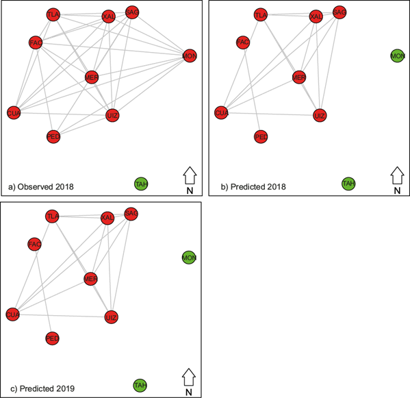
Fig. 10 Comparison between networks built with observed and predicted data for ⟨GOWE⟩ occurrence in 2018 and 2019.
In a previous study of temporal changes in the OWE at the three largest metropolitan areas in Mexico, Hernández-Paniagua et al. (2018) reported that 5 sites within the MCMA exhibited significant increases (p < 0.1) during 1993-2017. Here, we updated such analysis to 2018 and extended it to 10 monitoring sites located at different environments in order to determine whether the increase in the OWE annual magnitude occurred in a particular region or if it is spread within the whole MCMA. Overall, the increase in OWE annual magnitudes is consistent with the previous study of Hernández-Paniagua et al. (2018) for the inner sites MER, PED and TLA, but is no longer observed for the SAG and XAL. This is due to the difference in the period of assessment and arises from the OWE temporal-spatial evolution. Nevertheless, the OWE behaviour is consistent for inner and downwind sites which show significant increases in both studies.
4.6 Significance and future work
The results obtained show the potential of our approach to address future changes in the OWE spatial occurrence and O3 trends in response to future air quality control policies. It is very likely that emission control strategies targeting at VOCs reductions will help to reduce O3 not only on weekends but also on weekdays, which has been observed in VOC-limited environments similarly to that existing in the MCMA. By contrast, stricter policies aiming at reducing motor vehicles circulation on Saturdays could reduce traffic congestion and NOX ambient levels but will result likely in O3 increases as observed for Sundays. Due to the non-linear response of the O3 production system, the prediction of OWE occurrence could be improved in future studies by implementing spatial constraints in terms of network theory into multivariate models in order to produce more accurate predictions. Improving data capture of air pollutants at monitoring sites could also help to implement shorter-term modelling by generating information that could be used for alerting vulnerable populations during events of OWE occurrence.
While we used the most common method in air pollution (Mann-Kendall; Carslaw, 2019) to estimate OWE long-term trends within the MCMA, future work may include implementing additional approaches to compare the OWE trends quantification. Filters for pre-processing the OWE time series before applying our methodology could be implemented. For instance, the methodologies reported by Rodriguez et al. (2016) and Ramos-Ibarra et al. (2020) where the use of extreme values theory and estimation of the non-linear local trend can provide numerical OWE trend estimations. With the use of such methods, there could be other groups of monitoring sites with significant OWE trends, which would help to extend the forecast and network analysis presented here.
Additionally, a natural extension of this study is the application of our approach to monitoring data recorded at other cities, and trying to generalise the connectivity and structural properties reported here. In order to measure similarity, the Pearson’s correlation and comparison between networks built with it could provide other kind of information about the OWE spatial dependence. Additionally, random networks such as the exponential random graphs or scale free networks could be used to identify a generalisation of the OWE network model. Finally, this approach could be further used for establishing a model of spatial interactions with the aim of evaluating the OWE evolution in urban areas.
5. Conclusions
Numerical modelling is a powerful tool for investigating the evolution of chemical species in the atmosphere. However, due to extremely complicated urban canyon structure, lack of detailed description of the associated dynamic, thermodynamic and radiative processes within the urban canyon, small-scale turbulence, and lack of reliable meteorological analyses, it is a big challenge for numerical models to provide accurate predictions of urban chemical species near ground. Furthermore, numerical modelling can be costly. Therefore, statistical methods and long-term observations can be useful for studying urban scale phenomena.
The OWE occurrence can be considered as a drawback of larger reductions in NOX rather than in VOCs emissions during weekends, particularly from motor vehicles in urban areas with VOC-limited conditions. Within the MCMA, the annual OWE occurrence ranged typically between 40 and 60 % of the total weeks during 1994-2018. Significant increases were observed in the magnitude of OW1 and OW3 with the largest growth rates occurring at downwind sites. By contrast, non-apparent trends in the OWE magnitude were observed at upwind and fringe sites for OW1 and OW3 and for all sites for OW2 apart from the PED downwind site. This highlights the importance of implementing effective strategies for controlling O3 precursor emissions.
The concept of GOWE for a metropolitan area was integrated with trend, prediction and network analyses, and allowed the quantification of spatio-temporal variations in the OWE occurrence within the MCMA. The GOWE showed increases in the frequency of occurrence from 0.2 to 0.8 from 1994-1998 to 2014-2018. All the GOWE networks built for the MCMA showed the property of small world, implying that the magnitude of OWE occurrence was similar between monitoring sites both close and distant. It can be hypothesized that when the GOWE occurs, the existence of the largest cliques of equal size or greater than half the number of nodes in the corresponding network suggests the dominance of VOC-limited conditions within most of the study area.
The GOWE approach can be useful to approximate the identification of O3 chemical production regimes when inventory data and VOCs measurements are not available to be used in photochemical model simulations. Furthermore, the requirements both of human and computing resources often limit the use of detailed chemistry-transport models which are not required when applying GOWE analyses. Therefore, this approach may allow the study of the O3 production system in other cities or geographical regions with a representative spatial distribution of monitoring sites.
Finally, predicted networks suggested that the OWE will continue spreading over the MCMA. The method presented here proved to be a reasonable first approach for exploring relations between structures of OWE networks and their spatial and temporal interaction. Further work could include analyses on shorter time scales than a year and the comparison with data obtained for other cities in an effort to improve the evaluation and prediction of outcomes from air quality control measures aimed at reducing air pollution levels.