


 nueva página del texto (beta)
 Inglés (pdf)
 Artículo en XML
 Referencias del artículo
 Enviar artículo por email
 Citado por SciELO
  Similares en
SciELO
Similares en
SciELO 
 Permalink
1. Introduction
Despite the difficulties inherent to drought conceptualization and the establishment of parameters for the respective assessment and evaluation, consensus has been achieved on some of the major issues. First, there is more agreement regarding the definition of drought, despite slight nuances (Mishra and Singh, 2010). At present, drought is almost unanimously assumed to be a prolonged negative anomaly with respect to normal conditions of precipitation and water availability. The fact that drought is defined as an exceptional accumulation of anomalies over time is what allows droughts to occur anywhere in the planet, even in the wettest climates. But this is also what makes the phenomenon a natural hazard that can generate significant impacts due to interruption of the usual climatic rhythms, forcing societies to accordingly adjust their behavior. Also, there is consensus about the essential parameters to be assessed for appropriate characterization of drought, naturally derived from the phenomenon’s definition. Those parameters are duration or length (implying definition of onset and end of the dry sequence first), intensity and severity, which can be measured through several variables or indicators.
Following Mishra and Singh (2010), who adapted the contributions of Dracup et al. (1980), the basic set of parameters for drought characterization comprises the following (see Fig. 1):
Drought initiation time (ti): the start of the anomalous dry period.
Drought termination time (te): the time when the water shortage becomes sufficiently slight so that drought conditions no longer persist.
Drought duration (Dd): the period between the initiation and termination of a drought.
Drought severity (Sd): indicates a cumulative deficiency of a drought parameter below the critical level.
Drought intensity (Id): the average value of a drought parameter below the critical level. It is measured as the drought severity divided by the duration.
In addition, some authors have suggested the minimum value of the dry run (Xmin) as another expression of drought magnitude or severity, indicating the peak of the drought sequence (Hisdal and Tallaksen, 2000).
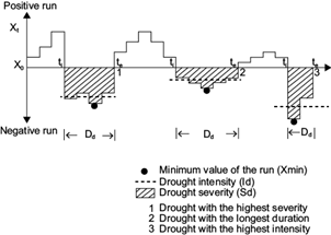
All the months comprised between the initiation and termination times are part of the same drought, also referred to as a “dry run”, “dry sequence” or “dry period” interchangeably in the cited specialized literature.
In a second stage under analysis, the different dry runs that occur in the time series of a particular place are described. Consideration of all these parameters would enable the respective drought hazard to be analyzed by expressing the probability of occurrence of the specific durations and magnitudes. This is the aim, for example, of the Drought Frequency Index (DFI) per González and Valdés (2006) or the work of Yusof et al. (2013) and Bonacorso et al. (2013).
In the aforementioned literature there is also a consensus about the necessity of indices for drought identification and monitoring and about the requirements they should meet. In this regard, it is essential for indices to reflect the definition of drought and that they be universal, standardized and comparable between different places. If possible, indicators should be also as simple and data-undemanding as possible, so that they can be applied by many observatories.
Finally, there is also agreement about recognizing the existence of different types or levels of drought: meteorological, edaphic, hydrological, agricultural, socio-economic, etc., each of which should have its own specific set of indicators (Wilhite and Glantz, 1985; AMS, 2004; WMO-GWP, 2016).
Since the mid-20th century, the compilation of these indices has evolved considerably. A number of advantageous and useful ones have been listed in very thorough reviews of the subject (Heim, 2002; Keyantash and Dracup, 2002; Mishra and Singh, 2010, 2011; WMO-GWP, 2016). Among them, the Palmer Drought Severity Index (PDSI) (Palmer, 1965; Karl, 1986; Guttman, 1991, 1998), the Standardized Precipitation Index (SPI) (McKee et al., 1993, 1995) and derivatives such as the Standardized Precipitation-Evapotranspiration Index (SPEI), are the most used and endorsed.
The first one uses the soil-water balance; it is undoubtedly the most sophisticated existing index and one of the most data-demanding. Along with its particular suitability for the field of agriculture (less so for other sectors fed with regulated water) and high local calibration and validation needs, this has limited its dissemination primarily to the USA, where it was developed.
The SPI has almost the opposite characteristics: it is very data-undemanding and rainfall (or runoff) is its only source of information. Also, its formulation is very simple (Tatli, 2015) and does not require local calibration. These features have made it the most universally used index in recent times. Indeed, since the Lincoln Declaration on Drought Indices (2009), the World Meteorological Organization has recommended its use in all regional meteorological services and has even produced a guide for users of this index (WMO, 2011).
However, no index has yet been able to reflect the phenomenon of drought in a totally appropriate manner, which justifies the continual modifications of existing indices and constant proposals for new ones meant to overcome the drawbacks of preceding ones.
Noteworthy, among the changes is the Modified Drought Index conceived by Pietzsch and Bissolli (2011), designed to overcome the two major drawbacks of the SPI in arid areas: the difficulty of fitting a suitable model for rainfall and the existence of multiple months without any precipitation (zero values). Also relevant is the contribution of the Multivariate Standardized Precipitation Index (MSPI), which seeks to solve the SPI’s need for multiple timescales by combining them all (Bazrafshan et al., 2014).
Outstanding among the new proposals are those that include evapotranspiration in the formulation. This enables inclusion of both water loss from soil and temperature variability, increasingly important in view of the global warming phenomenon. One of the first proposals in this sense is the Reconnaissance Drought Index (RDI) proposed by Tsakiris and Vangelis (2005) and widely used since its formulation (Tsakiris et al., 2007; Asadi Zarch et al., 2011; Khalili et al., 2011; Kousari et al., 2014). This index uses the classic ratio between precipitation and evapotranspiration (the long-established aridity index) for a given period. In the last stage it is normalized and standardized in the same way as the SPI.
The Standardized Precipitation Evapotranspiration Index (SPEI) (Vicente-Serrano et al., 2010) appeared later. Mathematically, it is very similar to the SPI, though based not only on precipitation but also on evapotranspiration.
The Water Surplus Variability Index, which encompasses the full soil-water balance (Gocic and Trajkovic, 2014), may be considered a continuation or improvement of the two previously mentioned indices.
Our work is along this line and proposes a new index for the analysis and monitoring of meteorological drought and more specifically rainfall drought. Indeed, monthly rainfall is the only variable used in the formulation. The emphasis on meteorological drought is justified by the fact that it is the earliest observable type, triggering the other types, for which it is to a certain degree anticipatory.
Rainfall drought is also the only truly natural type, not influenced by water and land use management, which are included in all the others. Also, analysis of the strictly natural phenomenon allows the effectiveness of drought policy and management to be evaluated by confronting natural drought and the respective impacts. Indeed, the distinction between natural and anthropogenic aspects of drought is required by the Water Framework Directive (articles 4.6 and 11.5, Water Framework Directive 2000/60). The implementation of certain relevant legal provisions in the area of insurance requires this distinction as well (EC, 2013).
The use of rainfall as the only source of information for preparation of the index is motivated by its status as a strictly natural variable and as stated its relatively high availability anywhere in the world and above all its fundamental role in drought generation, as it is the variable with the highest temporal variability of all potential participants. Indeed, even papers that include indices using temperature or derived parameters such as evapotranspiration declare that the greatest responsibility for drought genesis lies in the precipitation variability, and that very little can be attributed to temperature variability (Vicente-Serrano et al., 2010; Asadi Zarch et al., 2011; Khalili et al., 2011). These statements are particularly appropriate for arid and semiarid environments, which are precisely those in need of more and better drought monitoring indices, and where conventional indices present greater deficiencies (Wu et al., 2007; Pietzsch and Bissolli, 2011).
Among the indices like the one we propose (rainfall drought indices meant to be universally applied, with a simple formulation and requiring little information), the SPI has become the most used (McKee et al., 1993, 1995; Guttman, 1999; Lloyd-Hughes and Saunders, 2002). Its widespread dissemination can be attributed to its undeniable advantages (straightforward calculation, undemanding and standardized) thereby also making it universally comparable.
The multi-scale feature can be presented as an advantage of the SPI index, in so far as each scale allows for describing the drought conditions that trigger each resulting problem; each scale is therefore useful for a different application: meteorological, agricultural, hydrological, etc. (Lloyd-Hughes and Saunders, 2002). It offers multiple temporal aggregation possibilities; the user can choose the appropriate one.
However, this feature can be a limitation because it makes it impossible to establish the actual duration of each drought run, an essential feature for defining this particular natural risk and predicting its continuation or end. Moreover, some authors have pointed out how multi-scale prevents comparison between droughts that occur at different timescales (González and Valdés, 2006), also revealing that in certain timescales, such as 24 months, the method does not produce valid results (Guttman, 1999).
Besides this major limitation, two others are also particularly significant. First, the existence of places where it is not possible to find a model that fits the rainfall data prior to standardization. In Europe, this problem has been highlighted in various regions, including some areas of the Mediterranean (Lloyd-Hughes and Saunders, 2002; Bonaccorso et al., 2013). Second, the index’s inadequacy for short timescale application in climates where zero precipitation values are frequent, such as semiarid or Mediterranean regions during the summer season (Wu et al., 2007; Pietzsch and Bissolli, 2011).
With the aim of preventing all these problems, we propose a new drought index, the Drought Exceedance Probability Index (DEPI). First, the foundations of the new index and its calculation will be explained; second, its suitability for reflecting drought and its compliance with the objectives will be verified; next, its comparative advantages and complementarities will be presented; and finally, the main conclusions will be drawn. Prior to this, the study area and data used are presented in section 2.
2. Data
For application of the DEPI index, the monthly precipitation from 11 cells of the Climate Research Unit CRU TS vs. 4.01 grid was used. The centers of these cells are represented in Figure 2, corresponding to many different parts of the world and encompassing most of the world’s climates.
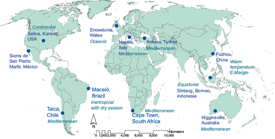
The CRU TS datasets pertain to the Climate Research Unit (University of East Anglia). This is a gridded product which provides data at a spatial resolution of half a degree in latitude and longitude, on a monthly basis from January 1901 to December 2016. The database values were subject to extensive quality control and homogenization processes (Harris et al., 2014).
The period between 1901 and 2015 was used for the analysis. It is long enough to be considered statistically significant and to encompass droughts of different lengths and intensities.
3. Calculation of the DEPI index
3.1 Initial notions
Rainfall drought indices are normally resolved by accumulating precipitation anomalies measured over normal rainfall values. In a later step, the accumulated anomalies are standardized with the aim of making them comparable between different parts of the world. This implies: (a) choosing a starting time scale; (b) establishing a benchmark to express what is considered the normal rainfall value for a certain period; (c) calculating the anomaly of the period from the normal value; (d) generating a procedure for accumulating the successive anomalies; (e) standardizing the values of accumulated anomalies, and (f) once all this is done and the standard values attributable to each of the months of the series are calculated, drought intensity thresholds are established to characterize each of the months.
In the case of the index we propose, these steps are covered as follows:
The input data used are monthly rainfall, as they have an appropriate level of aggregation for most existing climates.
The selected baseline to define normal monthly rainfall is the median. Most of the other indices, such as the SPI, use the average. The median was chosen because it is a valid central tendency measure for any climate, compared to the average, which in many types of climates, such as the Mediterranean and arid and semiarid ones, lacks the capacity to reflect normal conditions. In such climates monthly precipitation series are always skewed, with the highest frequencies at the lowest values, but with a few cases of very heavy rains that raise the average well above the most frequent values. As a result, the average always overestimates normal water supply conditions, while the median reflects them more accurately (Alfonso et al., 2019).
To evaluate the water deficit or anomaly experienced each month, the difference between total monthly rainfall and the median for that particular month is used.
It is in the process of anomaly accumulation (crucial for identifying the length of dry runs) where the greatest difficulties for drought index formulation occur. The mere accumulation of successive anomalies, despite its impeccable logic, leads to aberrant results. This is because precipitation is a variable that has a very sharp lower limit of 0, while no upper limit exists. This causes the positive anomalies to be systematically higher than the negative ones, so that after a certain accumulation the former annul the latter, which always results in rising positive accumulated anomalies. In such circumstances, only the configuration of ascending and descending sections in the series of accumulated rainfall anomalies allows identification of wet and dry sequences. It is nevertheless impossible to draw precise boundaries between them or quantify the intensity of drought. To prevent this problem, the SPI sets a priori durations of three, six, 12, 24, 48, etc. months and analyses drought for these durations, accumulating precipitation in each of these time scales and setting their level of abnormality with respect to the value considered normal for each case. With this system, it is directly assumed that each user can choose the most appropriate timescale for the final purpose. However, the downside is that the true length of the dry sequence under study cannot be properly demarcated with this method. The index we propose solves this key issue by accumulating successive rainfall anomalies but stopping and restarting the accumulation each time a new negative anomaly appears if the preceding accumulation is positive. The preceding surpluses thus do not mask the new dry month, which would occur if the accumulation continued (see the calculation procedure in more detail in section 3.2). This method is logical because, strictly speaking with respect to rainfall, any month recording a negative rainfall anomaly can be considered a dry month, regardless of the previous circumstances. Consequently, that month is the beginning of a new dry sequence whether or not the previous months have registered a precipitation surplus. This methodology solves the aforementioned problem of accumulation of surpluses and makes it possible to identify the real duration of each dry sequence (see Fig. 3).
For the standardization of cumulative anomalies, conversion into z-scores is one of the most-used solutions. This ensures expression of the anomalies in a standard and universally comparable score. Also, z-scores are linked to probability of occurrence values for the cumulative anomalies they come from, though only if they fit a normal distribution well. Since that fit is not always perfect, we replaced this standardization method by assigning exceedance probabilities to the values of cumulative monthly anomalies. The units in which our new index is expressed are consequently the empirical exceedance probabilities of the sample’s cumulative anomalies, calculated using the plotting position method (Weibull, 1939; Makkonen, 2006). The fact that the exceedance probabilities oscillate between 0 and 1 makes different data series comparable, thereby ensuring standardization. Also, since these are probabilistic values, they mark the uniqueness of the phenomenon for each month of the series, so that more severe droughts are closer to probability 0 and vice versa.
The thresholds of drought intensity are easily identifiable in this index since their values are comparable to probabilities of occurrence. If a long series of rainfall data is used, these values are directly related to empirical return periods, which are the most common magnitude in the field of natural hazards for establishing levels of intensity and risk. The thresholds proposed to characterize drought severity for this index are shown in Table I and are in line with the most used return periods for similar indices.
Table I DEPI levels of drought intensity.
| DEPI values (probabilities of exceedance) | Drought severity level | % months of a series within the interval | Return period (years) |
| DEPI≥0.5 | Wet conditions | 50 | 2 |
| 0.5>DEPI≥0.16 | Mild Drought | 34 | 6 |
| 0.16>DEPI≥0.07 | Moderate Drought | 9 | 15 |
| 0.07>DEPI≥0.02 | Severe Drought | 5 | 20 |
| DEPI<0.02 | Extreme Drought | 2 | 50 |
3.2 Calculation of the index
The index calculation is performed through the following successive stages:
In the first stage, the rainfall anomalies of each month of the series are calculated from the expression:
where P i is the precipitation of the month i and P MEDi is the median precipitation of the month i for the whole study period. See the second graph of Figure 4 for an example of calculation of these monthly anomalies.
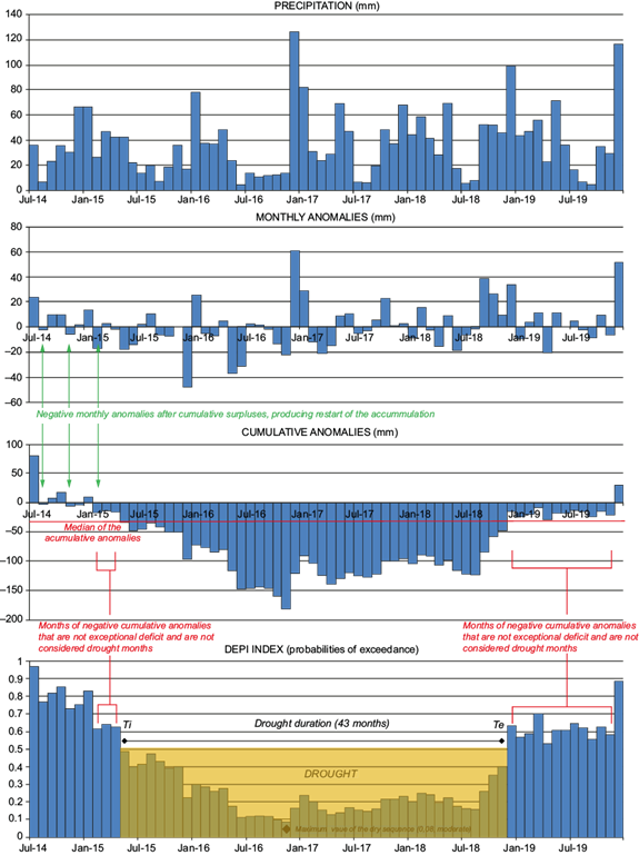
Fig. 4 Implementation of the Drought Exceedance Probability Index (DEPI) in the precipitation series of Ankara, Turkey, 1915-1918.
In the second stage, cumulative rainfall anomalies are calculated from the first month of the series (see third graph in Fig. 4). Each monthly rainfall anomaly is added to the accumulation of the previous months, with just an exception: every time that a negative monthly anomaly is found in a month in which the cumulative anomalies is positive (because there has been an accrued surplus over months), the accumulation is restarted in that particular month. In that month, the value of the cumulative anomalies is exactly the negative monthly anomaly of that month (see green arrows in Fig. 4). With this, the index calculation is emphasizing the fact that there is a rainfall deficit, regardless of the previous accumulated surplus.
After this restart, the regular addition of anomalies continues month by month. Even if cumulative anomalies become positive again after subsequent accumulations, monthly anomalies continue to be added until a new negative monthly rainfall anomaly is found. Obviously, a new restart occurs at that point as described above.
The methodology is therefore a continuous addition that stops whenever there is a monthly negative anomaly after a period of excesses, which precisely allows for prioritizing such anomaly. This avoids the effect of drought minimization resulting from the accumulation of surpluses which characterizes many of the most commonly used indices (Pita-López, 2007).
Consequently, the calculation of this second phase corresponds to the expression:
where APAc i is the rainfall cumulative anomaly of the month I; r is the value that marks the start of the dry season and follows the expression r = max{k: 1 ≤ k ≤ i, AP k < 0, APAc k-1 ≥ 0}.
Note that if AP i < 0 yAPAc i-1 ≥ 0, then r = i and as a result APAc i - AP i , marking the beginning of a new dry sequence.
Finally, in the third stage it is necessary to sort the monthly series of cumulative rainfall anomalies calculated in the previous stage from lowest to highest, namely, from the months with the largest negative cumulative anomalies or deficits, to the months with the largest positive ones or surpluses. This is necessary to obtain the empirical probabilities of exceedance corresponding to each month of the series. Once sorted, the probability of exceeding the event observed in each month is calculated using the Weibull (1939) method:
where PexcedAPAci is the empirical probability of exceedance of the month i, namely, the DEPI of month i; M APAci is the position of the rainfall cumulative anomaly of the month i in the sorted series, from lowest to highest cumulative anomalies, with M = 1 being the largest negative cumulative anomaly or largest observed deficit, and n is the total number of months in the series.
Hence, the DEPI for a given month is literally the probability of exceedance attributable to its cumulative rainfall anomaly, calculated as described above. This implies that it is a standardized value, therefore universally applicable and comparable between different series from different parts of the world. Also, being a probability value, it contains an estimate of the hazard.
According to this formulation, the series will always have half of the months marked as wet sequences (DEPI > 0.5) and half of the months marked as droughts (DEPI < 0.5), with the median value of the cumulative anomalies as the tipping point between the two (see red line in Fig. 4). This means that some negative cumulative anomalies will not be marked as droughts if they are not below the median, because they will not be considered exceptionally bulky deficits (see months in brown square brackets in Fig. 4).
The essence of the index, and its fundamental mark of identity over similar ones, is that it restarts the calculations of cumulative anomalies whenever a new dry month (AP i < 0) arises in the context of a surplus period (with APAc i-1 ≥ 0). This ensures the proper identification of dry runs of different lengths from a single calculation of the index.
Figure 4 shows an example of application of the DEPI to one of the greatest droughts recorded in Ankara, Turkey (1915-1918), also showing how the method allows clear definition of each dry sequence from its most important parameters: drought initiation time (ti), situated in the first month with a probability of exceedance equal to or below 0.5; drought termination time (te), situated in the first month with a probability of exceedance over 0.5 after each drought event; drought duration (Dd), which is the number of months located between ti and te; drought severity of each month (Sd), which is the monthly DEPI value itself; drought intensity (Id), which is the average value of all the DEPI values within the dry sequence, and the minimum value of the index (DEPImin) within the drought period, which is the peak of highest severity.
We stress that resolving calculation of the index is doable with standard numerical/statistical packages. At http://alojamientosv.us.es/climatemonitor/news/ an R code for application of the index to the user time series is available.
4. Application of the DEPI to the selected time series (1901-2015)
The DEPI was computed for monthly rainfall data in the analyzed series from 1901 to 2015 and plotted in Figure 5. The results are very different among the eleven series and cannot be easily attributable to their different rainfall features. To facilitate interpretations, Figures 6 and 7 show a summary of some characteristics defining the dry periods identified with the DEPI index in the selected points.
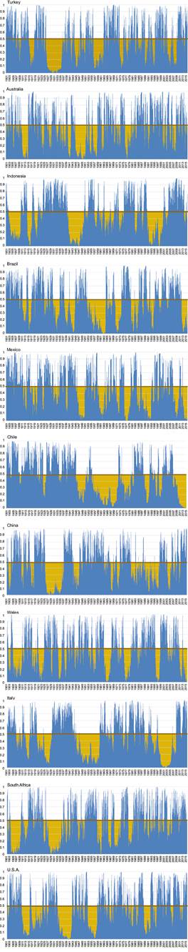
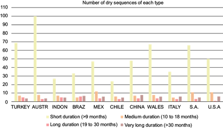
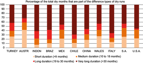
Fig. 7 Percentage of the total dry months that are part of droughts of the different duration categories.
A few series like the one in Italy, the one in China and the one in Chile, show one or two droughts of much longer duration than a decade, in which the anomalies increased continuously. The DEPI index is nevertheless able to also capture the shortest runs in them, however intense. Other series like the ones in Australia, Wales, Mexico or South Africa develop more dry runs of short duration, recovering more quickly from intense deficits, though falling into them more frequently (see Fig. 5).
The seasonality of the series’ precipitation, tested using the Rainfall Seasonality Index by Walsh and Lawler (1981), shows no connection with the DEPI index behavior and derivative parameters (number of dry runs, respective lengths, etc.), nor do any of the measures of variability for rainfall regimes utilized: monthly variation coefficients and inter-annual variation coefficients. This indicates that the overall type of rainfall regime does not condition performance of the index.
However, there is a significant positive correlation between the month-to-month rainfall persistence of the series (measured following Ledbetter, 2012) and the number of long and very long dry runs they show in their DEPI series, although the opposite statement is not valid (see Fig. 8). Likewise, the higher the one-month lag autocorrelation of the rainfall time series, the more prone to developing long dry runs it shows (Fig. 8) and vice versa. This indicates that monthly rainfall inertia shapes more sustained behavior in the drought index in the used data points. However, this particular analysis should be performed with more than 11 points to confirm the strength of such connection, since it is important to determine if a particular monthly rainfall behavior points to a distinctive kind of drought sequence (longer, shorter, more intense, more attenuated, etc.).
Fig. 8 Connection between the type of dry runs observed in the selected series and their month-to-month rainfall persistence and one-month lag autocorrelation.
Despite these nuances, the calculated time series of the DEPI do not differ substantially in characteristics among themselves. In each of the eleven generated DEPI series, a similar number of dry sequences reaching the different drought severity thresholds defined in Table I is found; this is a satisfactory result for an index that is meant to reflect probabilities of the generated deficits. These aspects suggest that the index is suitable for delineating droughts in very different climatic domains.
5. Comparison of the DEPI and the SPI. Potential benefits and complementarities
The main contribution of the DEPI would be the accurate establishment of drought duration and associated cumulative severity, two of the most difficult and less successful aspects to establish in the field of drought indices, particularly the simpler and less data-demanding ones.
Given that the SPI has demonstrated capacity to show different drought dynamics which can be experienced in a given place, with great simplicity, we shall use its comparison with the newly proposed DEPI to demonstrate the latter’s suitability for establishing the onset, end and duration of dry sequences.
Figure 9 and Table II, which depict the existing relationships between DEPI and SPI at different time resolutions, offer a first sample of this contribution. There is generally a very good correlation between the values of both indices at all temporal resolutions, even when all the monthly values are included in the calculations, including the wet ones. The best correlations occur with SPI 36 or SPI 48 in series with a tendency to long dry runs registered with the DEPI, such as in Indonesia, China or Italy, and with SPI 6 for those with short ones like Australia. The other examples lie in between these two situations and show very good correlations between DEPI, and SPI 12 and SPI 24.
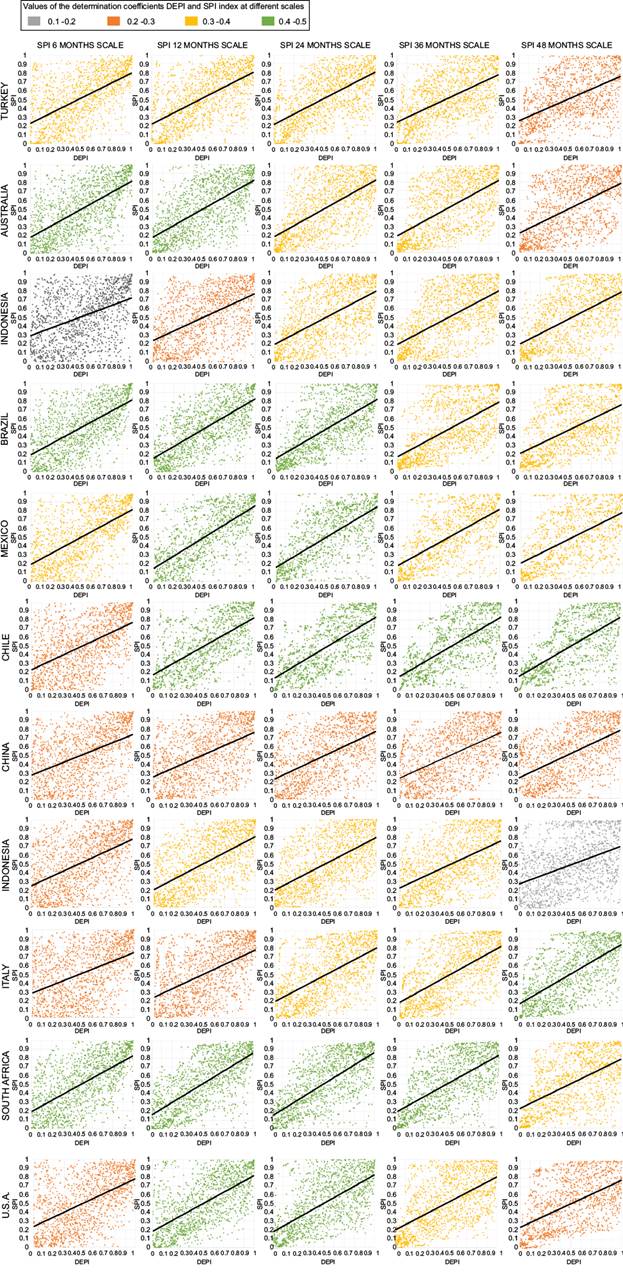
Table II Relationships between the DEPI and SPI at different scales in the eleven samples. Pearson correlation coefficient values (r).
| Turkey | Austria | India | Brazil | Mexico | Chile | China | Wales | Italy | South Africa | USA | |
| SPI 6 | 0.59 | 0.64 | 0.43 | 0.65 | 0.62 | 0.54 | 0.46 | 0.53 | 0.45 | 0.63 | 0.54 |
| SPI 12 | 0.61 | 0.65 | 0.52 | 0.7 | 0.71 | 0.65 | 0.53 | 0.59 | 0.53 | 0.7 | 0.63 |
| SPI 24 | 0.63 | 0.63 | 0.59 | 0.68 | 0.68 | 0.69 | 0.51 | 0.6 | 0.6 | 0.71 | 0.64 |
| SPI 36 | 0.58 | 0.61 | 0.6 | 0.61 | 0.62 | 0.67 | 0.52 | 0.55 | 0.63 | 0.63 | 0.59 |
| SPI 48 | 0.53 | 0.54 | 0.58 | 0.55 | 0.56 | 0.66 | 0.54 | 0.44 | 0.65 | 0.55 | 0.54 |
To better show the adequacy of the DEPI for establishing drought onset, termination and consequent duration, both indices are visually contrasted in some of the most important droughts of two of the selected points. This required the homogenization of both indices, so they are directly comparable visually, with the SPI values expressed in probabilities. The different SPI values, which are z-scores, were therefore replaced by their corresponding probabilities of exceedance derived from the normal distribution, to which the index fits by definition. Results for two notable droughts in the series of Wales and the USA are shown in Figures 10 and 11.
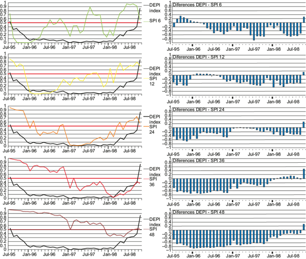
Fig. 10 Multiple timescale comparison between the DEPI and SPI applications to the 1995-1998 drought event in Snowdonia, Wales.
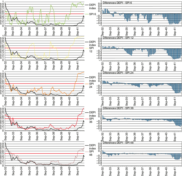
Fig. 11 Multiple timescale comparison between the DEPI and SPI applications to the 1933-1941 drought event in Kansas, USA.
In the example of Wales, the DEPI shows a noteworthy advantage. In this three-year long dry run, short-term SPI indices (six and 12 months timescales) produce good results for the time of drought onset, but do not mark its end, while longer duration indices (36 or 48 months) are valid for the end but not for the beginning of the dry run. Reinforcing these arguments, if the DEPI and SPI are compared in this dry sequence alone, low to negative correlations are found with all SPI scales except for SPI 12 and SPI 24, for which the respective Pearson coefficients are 0.67 and 0.83.
Similarly, in the very long drought in Kansas, USA, it is evident that the SPI in the short timescales is unable to adequately reflect the residual dryness of the final couple of years, in which the created deficit has not fully recovered even though the months are wetter. Also, the precise onset of this drought is not clear for the SPI and depends on the scale. The more the time scale increases, the higher the degree of harmony between the SPI and DEPI, until a nearly perfect congruence is found from the 24-month resolution. Comparing the DEPI and the SPI in this dry sequence alone, non-significant correlations are found with all the SPI scales except for SPI 36 and SPI 48, for which the Pearson coefficients are 0.61 and 0.72, respectively.
Indeed, in the dry runs of all the samples it was observed that the series of SPI values start to converge with the DEPI ones at around months six, 12, 24, 36 or 48 of every DEPI dry run, depending on the respective SPI scale applied (from six to 48). This reveals the different levels of inertia of each SPI time scale, so that the use of each SPI time resolution determines not only the length assigned to a specific drought episode (which is different from one SPI timescale to another), but also the location of the drought episode itself, since both the beginning and the end are shifted.
The right side of Figures 10 and 11, which show the absolute differences observed between the DEPI and the SPI for the 6, 12, 24, 36 and 48-month reference timescales in the previously analyzed events, also depict that phenomenon very well. Two facts are remarkable:
No SPI is valid for the entire length of the drought; the SPI estimates for short scales are valid for the beginning of the drought but not for the end; the estimates for longer scales are valid for the end but not for the beginning of the drought.
Especially noteworthy is that the smallest differences between the DEPI and the SPI are generally found at the drought duration corresponding to the scale of the respective SPI. This would be a good indicator of a better capacity of the DEPI to reflect the real duration of the drought and its severity.
Apart from the described validity of the DEPI for depicting the evolution of long, creeping droughts, it shows great accuracy for detecting very important flash droughts as well, namely events where for a short period (several weeks or a month) the phenomenon’s severity increases in several categories (Chen et al., 2019).
For example, in January 1984 in Mexico a moderate drought was undergone (see Table I for categories) just for that month, coming right after a very wet sequence; the SPI scales beyond SPI1 naturally do not reflect this sudden drought until later months, if the deficit continues. Precisely the same thing happens in May 1934 and May 2000 in the series for Australia, or in May 1987 in the Brazil series, or June 1901 in South Africa, to mention just some of the examples found.
These statements do not call into question the already broadly proven value of multi-scalar drought indices. The multiple scales of the SPI (and derived and similar indices) are designed to overcome the drawback that there is no single drought index that can capture all the varied set of drought impacts resulting from the different drought types: meteorological, soil, agricultural, hydrological, hydrogeological and socioeconomic (Wanders et al., 2017). As pointed out by Vicente-Serrano et al. (2010), the time period from the arrival of water inputs to availability of a given usable resource differs noticeably and the time scale over which water deficits accumulate becomes important for distinguishing impacts.
Indeed, when the SPI is computed for shorter accumulation periods (one to three months), it relates to instant impacts such as decreased soil moisture, snowpack and flow in small catchments; but when the SPI is calculated for medium accumulation periods (around six to 12 months), it can be used as an indicator for reduced stream flow and reservoir storage (EC, 2020). Longer timescales (SPI24 and beyond) have been found to correlate significantly with groundwater levels and total water storage in aquifers during drought (Leelaruban et al., 2017; Cammalleri et al., 2019).
The DEPI is also very convenient for accurately delimiting in time and tracking the evolution of the natural deficit that generates the rest of the cascading effects with a single straightforward calculation.
6. Conclusions
This paper has presented a new rainfall drought index, the DEPI, calculated from time series of monthly precipitation data. It has described the development of the index and its application to the monthly precipitation series (CRU TS database) for eleven points around the globe with different regimes for the period 1901 to 2015. None of the developed series showed artefacts and all showed comparable results in terms of types, numbers and lengths of the dry sequences identified.
The calculation of the SPI in the same locations and for the same period allowed for comparison between the two indices. The results show that the DEPI is more effective for unquestionably establishing the onset, end and total duration of a purely natural drought. For the long-term DEPI droughts, the SPI short timescales (e.g., SPI 1 to SPI 12) are useful for identifying the beginning, but not the end. This occurs because the calculation of the SPI at those scales stops considering the situation as a shortfall as soon as a limited number of months (equivalent to the timescale) are not significantly dry anymore, even if the previous ones already created a severe deficit.
On the contrary, the long timescales (SPI 24, SPI 36, etc.) reflect the end of the dry sequences but not their onset, for the opposite reasons: it is necessary to have many months with deficit for it to start becoming sufficiently anomalous.
However, the DEPI shows great ability to reflect the actual duration of the drought in all cases because it restarts the accumulation of negative anomalies anytime they reappear, though only marking their exceptional accumulation. The deficit disappears only when a following chain of wet months amount to the accumulation of negative anomalies.
It is therefore a particularly suitable index for describing long-term droughts, the most important ones to be monitored and controlled in climates such as the Mediterranean or other semiarid ones. Yet it is equally valid for defining short dry runs and is a good alternative or complement to the use of other undemanding drought indices.
A number of extensions to this work are possible:
First, the authors are extending its calculation worldwide and sharing the gridded results via the Global Climate Monitor (www.globalclimatemonitor.org), a web geo-viewer developed by the same research team and also based on CRU TS data, among other sources. This viewer is available to visualize and share global climatic variables and indices (Camarillo et al., 2019).
The ability of this new index to identify the most interesting features of drought will be leveraged. For example, the team is analyzing and characterizing the hazard by identifying the type of curve that fits the low values of the DEPI for different locations and time series. It is an efficient method for classifying the types of drought that each climate (or each region) is more likely to register, in the same way as is frequently done for flood modelling (Han, 2011).
It would also be desirable to extend the analysis presented in this paper to the series of future climate change scenarios. This would require the gradual adaptation of what are considered normal rainfall conditions, because very few places on the planet record stationarity or stability.
Finally, exploration of the possibilities and methods of prediction for the index values in the immediate future could be of great interest for drought management.
Work on these issues is under way.

