


 nova página do texto(beta)
 Inglês (pdf)
 Artigo em XML
 Referências do artigo
 Enviar este artigo por email
 Citado por SciELO
  Similares em
SciELO
Similares em
SciELO 
 Permalink
1. Introduction
Climate change triggers severely negative effects on global water resources (Fares et al., 2016). In fact, changes in rainfall distribution have attracted so much attention because of the vulnerability of human activities to extreme hydrological events such as flood-producing rains and droughts (Kharin et al., 2007). These precipitation changes could also have a dramatic effect on agriculture (Yue et al., 2010.) Record-breaking rainfall events around the world during the last decade have had a severe impact on human society and the environment including agricultural losses and flooding (Lehmann et al., 2015). Changes in water availability or, more importantly, the shortage of water in the future could have negative impacts on hydropower generation as well on agricultural activities in Central America and Mexico (Karmalkar et al., 2011). Such is the case of the arid and semi-arid irrigated land areas (150 000 ha) in the state of Zacatecas, central Mexico.
The state of Zacatecas is one of the main providers of basic grains in Mexico, primarily dry beans (Cid et al., 2018) and corn, but several of its 34 aquifers are overexploited with a deficit of about 433 Mm3 per year (SEMARNAT, 2015). A better understanding of the spatial and temporal variability of precipitation over land, at local and regional levels, is necessary for advancing climate change research, as well as for estimating the potential impact of climate change on water resources (Nickl et al., 2010). Several studies suggest that precipitation trends vary over time and according to regions, although precipitation over land has generally increased in the north at 30° N over the past century and decreased over much of the tropics since the 1970s (IPCC, 2013). Recent studies on precipitation during the last 20 years suggest that the current climate is becoming wetter compared with the climate of the 1950s in North America (Huang et al., 2016). Precipitation at higher latitudes has generally increased notably over North America, Eurasia and Argentina (Trenberth, 2011).
Variations and trends of precipitation may be affected by quasi-periodic phenomena, that is, phenomena that happen repeatedly at irregular intervals. For instance, El Niño-Southern Oscillation (ENSO), the most important coupled ocean-atmosphere phenomenon, causes global climate variability in inter-annual time scales (Wolter and Timlin, 2011). Precipitation increases over northwestern Mexico during El Niño winters but decreases in the region around the Isthmus of Tehuantepec. A southward shift in the location of the subtropical jet stream also increases the number of cold fronts over the southern part of the Gulf of Mexico (Magaña et al., 2003). Research should nonetheless include the possible association between precipitation and periodic phenomena (Valdez-Cepeda et al., 2012) such as ENSO at local and regional levels. An interesting teleconnection between precipitation anomalies registered at the Litter River Watershed, Tifton, Georgia, USA and the ENSO 3.4 index of sea surface temperature was confirmed by Keener et al. (2010) through the wavelet coherence analysis.
Several studies suggest important relationships between ENSO and local or regional precipitation patterns (e.g., Magaña et al., 2003; Kane, 2009; Keener et al., 2010; Li and Chen, 2014), but a relation between ENSO and rainfall in Central Mexico (i.e., Zacatecas state) has not been reported. The aims of this study were therefore: (1) To cluster standardized anomalies of the monthly precipitation (SAMP) time series into groups that represent regions under the basis of similar precipitation regimes, (2) to generate regional SAMP time series using all the members (time series) for each cluster, (3) to identify important frequencies in each regional SAMP time series and possible connections with quasi-periodic phenomena, and (4) to detect coupling signals using each estimated regional SAMP and the MEI.
2. Material and methods
2.1 Precipitation data
Monthly precipitation data from 59 sites located within the state of Zacatecas, Mexico (Fig. 1) were analyzed. Table I provides information on location. Data sets were kindly provided by the Comisión Nacional del Agua, the official national institution in charge of recording climatic and meteorological data in Mexico. Time series of 34 years (1976-2010) were checked for outliers or missing values.
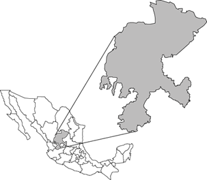
Table I Network of weather stations located within the territory of the Mexican Zacatecas state.
| Station | Station name | Latitude | Longitude | Meters above sea level | Cluster |
| 1 | Agua Nueva | 23º 46' 55'' | 102º 09' 39'' | 1932 | I |
| 2 | Boca del Tesorero | 22º 49' 20'' | 102º 57' 05'' | 2045 | III |
| 3 | Calera | 22º 54' 00'' | 102º 39' 00'' | 2192 | II |
| 4 | Estación Camacho | 22º 26' 26'' | 102º 22' 11'' | 1658 | I |
| 5 | Cañitas | 23º 36' 07'' | 102º 43' 53'' | 2025 | II |
| 6 | Caopas | 24º 46' 52'' | 102º 10' 16'' | 2000 | I |
| 7 | Cedros | 24º 40' 43'' | 101º 46' 26'' | 1763 | I |
| 8 | Chalchihuites | 23º 14' 27'' | 102º 34' 31'' | 2060 | II |
| 9 | Col. González Ortega | 23º 57' 22'' | 103º 27' 02'' | 2190 | II |
| 10 | Concepción del Oro | 24º 37' 16'' | 101º 23' 26'' | 1940 | I |
| 11 | El Arenal | 23º 39' 01'' | 103º 26' 52'' | 2016 | II |
| 12 | El Cazadero | 23º 41' 35'' | 103º 26' 50'' | 1898 | II |
| 13 | El Platanito | 22º 36' 43'' | 104º 03' 05'' | 990 | III |
| 14 | El Rusio | 22º 26' 34'' | 101º 47' 09'' | 2104 | II |
| 15 | El Sauz | 23º 10' 47'' | 103º 12' 26'' | 2090 | II |
| 16 | Excamé III | 21º 38' 58'' | 103º 20' 23'' | 1740 | III |
| 17 | Fresnillo | 23º 10' 22'' | 102º 56' 26'' | 2195 | II |
| 18 | Gral. Gpe. Victoria | 22º 23' 43'' | 101º 49' 52'' | 2183 | II |
| 19 | Gruñidora | 24º 16' 29'' | 101º 53' 05'' | 1825 | I |
| 20 | Huanusco | 21º 46' 01'' | 102º 58' 07'' | 1495 | III |
| 21 | Jerez | 22º 38' 31'' | 103º 00' 05'' | 2098 | III |
| 22 | Jiménez del Teúl | 23º 15' 18'' | 103º 47' 54'' | 1900 | III |
| 23 | Juan Aldama | 24º 17' 14'' | 103º 23' 34'' | 1995 | II |
| 24 | Juchipila | 21º 23' 14'' | 103º 06' 53'' | 1270 | III |
| 25 | La Bufa | 22º 47' 00'' | 102º 34' 00'' | 2612 | II |
| 26 | La Florida | 22º 41' 10'' | 103º 36' 09'' | 1870 | III |
| 27 | La Villita | 21º 36' 08'' | 103º 20' 13'' | 1790 | III |
| 28 | Loreto | 22º 16' 40'' | 101º 59' 15'' | 2029 | II |
| 29 | Malpaso | 22º 37' 05'' | 102º 45' 15'' | 2135 | II |
| 30 | Monte Escobedo | 22º 19' 32'' | 103º 29' 38'' | 2190 | III |
| 31 | Nochistlán | 21º 21' 55'' | 103º 50' 32'' | 1850 | III |
| 32 | Nuevo Mercurio | 24º 13' 38'' | 102º 09' 09'' | 1706 | I |
| 33 | Ojocaliente | 22º 24' 38'' | 102º 16' 09'' | 2050 | II |
| 34 | Pajaritos de la Sierra | 22º 39' 36'' | 104º 16' 38'' | 2660 | III |
| 35 | Palomas | 22º 20' 47'' | 102º 47' 48'' | 2030 | III |
| 36 | Pinos | 22º 16' 54'' | 101º 34' 47'' | 2408 | II |
| 37 | Presa El Chique | 22º 00' 00'' | 102º 53' 23'' | 1620 | III |
| 38 | Puerto de San Fco. | 23º 44' 01'' | 103º 23' 13'' | 2330 | II |
| 39 | Río Grande | 23º 48' 01'' | 103º 01' 36'' | 1890 | II |
| 40 | San Andrés | 23º 41' 55'' | 101º 55' 45'' | 2085 | I |
| 41 | San Antonio del Ciprés | 22º 56' 08'' | 102º 29' 14'' | 2145 | I |
| 42 | San Benito | 23º 54' 10'' | 101º 43' 07'' | 1955 | I |
| 43 | San Gil | 24º 11' 43'' | 102º 58' 36'' | 1810 | II |
| 44 | San José de Llanetes | 22º 54' 45'' | 103º 16' 43'' | 2176 | II |
| 45 | San Juan Capistrano | 22º 38' 39'' | 104º 06' 01'' | 2660 | III |
| 46 | San Pedro Piedra Gorda | 22º 27' 09'' | 102º 20' 49'' | 2032 | II |
| 47 | San Tiburcio | 24º 08' 50'' | 101º 28' 58'' | 1887 | I |
| 48 | Santa Lucía | 22º 26' 03'' | 104º 13' 00'' | 2252 | III |
| 49 | Santa Rosa | 22º 55' 34'' | 103º 06' 47'' | 2240 | III |
| 50 | Tayahua | 22º 07' 13'' | 102º 51' 46'' | 1549 | III |
| 51 | Teúl de González | 21º 27' 42'' | 103º 27' 59'' | 1900 | III |
| 52 | Tlaltenango | 21º 46' 54'' | 103º 17' 45'' | 1700 | III |
| 53 | Trancoso | 22º 44' 39'' | 102º 22' 10'' | 2190 | II |
| 54 | Valparaíso | 22º 26' 03'' | 104º 13' 00'' | 1890 | III |
| 55 | Villa de Cos | 23º 17' 26'' | 102º 20' 44'' | 2050 | II |
| 56 | Villa García | 22º 10' 10'' | 101º 57' 27'' | 2120 | II |
| 57 | Villa Hidalgo | 22º 20' 49'' | 101º 42' 55'' | 2167 | II |
| 58 | Villanueva | 22º 21' 43'' | 102º 53' 22'' | 1920 | III |
| 59 | Zacatecas | 22º 45' 39'' | 102º 34' 30'' | 2485 | II |
Note: clusters: I, semi-arid region; II, highlands region; III: canyons region.
2.2 Precipitation linear trends and anomaly time series
Precipitation time series are in general non-stationary and frequently present long-term trends. Identifying the trends and detrending the data are both of great interest and importance in data analysis. Moreover, detrending climate data is often a necessary step before meaningful spectral results can be obtained (Wu et al., 2007). Linear trends of the 59 precipitation time series were estimated through a linear regression analysis, considering this simple model:
where Y i is the i th monthly precipitation and X i is the i th month.
Before carrying out the fractal analysis with the power spectrum density approach, linear trends of the series were removed following Eq. (2):
where Y di is the i th detrended monthly precipitation.
After removing the trends, the standardized anomalies were computed simply by subtracting the sample mean and dividing by the corresponding sample standard deviation, as pointed out by Wilks (2006). The new time series were then referred to as “SAMP time series” and could be analyzed by using common statistical analysis and other approaches like the spectral analysis which uses several algorithms such as maximum entropy, autoregressive moving average, non-harmonic method, singular spectral analysis and the traditional Fourier analysis (Lana et al., 2005).
2.3 Cluster analysis
Cluster analysis is an effective statistical tool to find homogeneous climate regions based upon observed values of meteorological parameters (Unal et al., 2003; Mahlstein and Knutti 2010; Karmalkar et al., 2011). This approach groups data objects based only on information found in the data that describes the objects and their relationships. The goal is that the objects within a group be similar to one another and different from the objects in other groups (Tan et al., 2005). The greater the similarity within a group and the greater the difference between groups, the better or more distinct the clustering becomes (Tan et al., 2005). In this study, we used a tree clustering algorithm to join objects (i.e., SAMP) into successively larger clusters (i.e., regions under the basis of similar precipitation regimes). The 1-Pearson’s r (Everitt et al., 2011) was used as linkage distance and the Ward’s method was used as linkage rule.
The joining (or tree clustering) method uses the similarities or distances between objects when forming the clusters. Similarities are a set of rules that serve as criteria for grouping or separating items. The distances can be based on a single dimension or on multiple dimensions, with each dimension representing a rule or condition for grouping objects. In the case of the 1-Pearson’s r (Everitt et al., 2011) as linkage distance, low values mean that both involved elements are highly positively correlated, while two elements having low positive correlation are more distant from each other. The Ward’s method (Ward, 1963) is generally regarded as very efficient although it tends to create small-sized clusters (Unal et al., 2003) and uses an analysis of variance approach to evaluate the distances between clusters. This method defines the proximity or distance between two clusters as the increase in the squared error that results when two clusters are merged (Tan et al., 2005). The cluster analysis was performed in this research using Statistica v. 8.0 (StatSoft, 2007).
2.4 Fractal analysis
The temporal variation of natural phenomena has been difficult to characterize and quantify, which is why Mandelbrot (1982) introduced the fractal analysis. Time series can be characterized by a non-integer dimension (fractal dimension) when treated as random walks or self-affine profiles. These series can be treated as self-affine systems because they are invariant only under anisotropic magnifications (Bunde and Havlin, 2013). Self-affine systems are often characterized by roughness, which is defined as the fluctuation of the height over a length scale. For self-affine profiles, the roughness scales with the linear size of the surface by an exponent called the Hurst exponent (Turcotte, 1997). This exponent, however, only gives limited information about the underlying distribution of height differences (Evertsz and Berkner, 1995). The Hurst exponent as well as the fractal dimension measure how far a fractal curve is from any smooth function used to approximate it (Moreira et al., 1994). There are several approaches to estimate fractal dimension for self-affine profiles but we only used the power spectrum technique because it is very sensitive and is a good exploratory tool for real data (Weber and Talkner, 2001).
2.5 Power spectrum approach
Self-affine fractals are generally treated quantitatively through spectral techniques. The variation of the power spectrum P(f) with frequency f appears to follow a power-law (Turcotte 1997):
The power spectrum P(f) is defined as the square of the magnitude of the Fourier transform of the SAMP. Denoting SAMP as a function of time by Z(t), we have:
where t 0 and t 1 are the limits of time over which the series extend. The discrete version of Eq. (4) should be used for such a standardized anomaly sampled at discrete time intervals:
The next step is to obtain a relationship between the power β and the fractal dimension D. After considering the time series Z 1 (t) and Z 2 (t) separated by distance r and related by
it can be observed that Z 1 (t) has the same statistical properties as Z 2 (t), and since Z 2 is a properly rescaled version of Z 1 , their power spectral densities must also be properly scaled. We can then write:
It follows that
And
where D s denotes the fractal dimension estimated from the power spectrum and H is the Hurst exponent (see Valdez-Cepeda et al., 2003a, b, 2007).
Since the periodogram is a poor estimate of the power spectrum, we used the Welch method of averaging periodograms (Welch, 1967). We also used the “running sum” transformation to shift the slope by a factor of +2. The Hurst exponent and the D s (because of data-trace) had a slope between -1 and 1 on the log-log plot. Major modal contributors could then be identified in such a plot.
In order to obtain an estimate of the fractal dimension D s , one must calculate the power spectrum P(f) (where f, f is the wavenumber, and l is the wavelength), and plot the logarithm of P(f) versus the logarithms of f. This plot should follow a straight line with a negative slope -ß if the profile is self-affine (Valdez-Cepeda et al., 2003a, b).
The power spectrum approach involving the SAMP was carried out using the Benoit 1.3 software (TruSoft, 1997). The important frequencies of SAMP were estimated through the plot yielded by power spectral density Φ x (f) versus frequency, considering significant p ≤ 0.05 peaks.
2.6 Multivariate El Niño Southern Oscillation Index data
The ENSO is arguably the most important coupled ocean-atmosphere phenomenon causing global climate variability on inter-annual time scales (Wolter and Timlin, 2011). The MEI is calculated based on the six main observed variables over the tropical Pacific (Wolter 1987; Wolter and Timlin 1993, 1998). These six variables are sea-level pressure, zonal and meridional components of the surface wind, sea surface temperature, surface air temperature, and total sky cloudiness fraction. The MEI is computed separately for each of 12 sliding bi-monthly seasons (Dec/Jan, Jan/Feb, …, and Nov/Dec). After spatially filtering the individual fields into clusters (Wolter 1987), the MEI is calculated as the first un-rotated principal component (PC) of all six observed fields combined. This is accomplished by normalizing the total variance of each field first and then performing the extraction of the first PC on the covariance matrix of the combined fields (Wolter and Timlin, 1993). All seasonal values are standardized with respect to each season in order to keep the MEI comparable. A MEI database with a length matching our precipitation records (1976-2010) was downloaded from the National Oceanic and Atmospheric Administration website (http://www.esrl.noaa.gov) and used to couple it with each of the standardized anomaly regional means of the monthly precipitation time series. The MEI was used because it has been related to precipitation in several regions around the world and takes into account ENSO’s seasonality. For instance, precipitation was positively and significantly correlated with the MEI during the boreal winter (Nov-Apr), mainly in northeastern and northwestern Mexico (Méndez-González et al., 2009).
2.7 Wavelet coherence analysis
Wavelet analysis is a spectral method of decomposing a time series into time and frequency space. This allows the identification and analysis of dominant localized variations of power, i.e., where the variance of the time series is largest for a given frequency (Keener et al., 2010). Transferring the concept of the Fourier analysis, a wavelet power spectrum (WPS) can be defined as the wavelet transformation of the autocorrelation function (Maraun and Kurths, 2004). This can be implemented following the Wiener-Khinchin theorem (Maraun and Kurths, 2004):
where the brackets denote expectation values and WPS i (s) describes the power of the signal x(t) at a certain time t i on a scale s.
As in the Fourier analysis, the univariate WPS can be extended to compare time series, for instance, x(t i ) and y(t i ). One can define the wavelet cross-spectrum [WCS i (s)] as the expectation value of the product of the corresponding W ix (s) and W iy (s):
In contrast to the WPS, the WCS is a complex value (analogous to Fourier cross-spectra) and can be decomposed into amplitude |WCS i (s)| and phase Φi(s):
The phase Φ i (s) describes the delay between the two signals at time t i on a scale s.
A normalized time and scale resolved measure for the relationship between the time series x(t i ) and y(t i ) is the wavelet coherency (WCO), defined as the amplitude of the WCS normalized to two single WPS, is the following:
A value of 1 means a linear relationship between series x(t i ) and y(t i ) around time t i on a scale s. A value of zero is obtained for vanishing correlation.
Spurious peaks can occur for areas of low wavelet power due to normalization. Note the importance of estimating the expectation values of the single terms in Eq. (14). If they are not considered separately, numerator and denominator will equal each other, and the result will be identical to 1 no matter what the real WCO is. When computing WCO from observational data, one must thus smooth the numerator and denominator separately (Maraun and Kurths, 2004). In the current case, WCO was performed involving the MEI series and each of the three regional SAMP under the basis of a 95% confidence level. We used the MatLab code developed by Grinsted et al. (2004) for this purpose. The code is available at http://noc.ac.uk/marine-data-products/cross-wavelet-wavelet-coherence-toolbox-matlab.
3. Results and discussion
3.1 Cluster analysis
A cluster analysis was performed using the 59 SAMP time series with the aim of grouping them into successively larger groups (i.e., regions under the basis of similar precipitation regimes). The dendrogram (Fig. 2) revealed three clusters or regions (Table I) when using a linkage distance value of 1: (I) semi-arid region (11 out of 59 stations); (II) highlands region (27 out of 59 stations), and (III) canyons region (21 out of 59 stations).
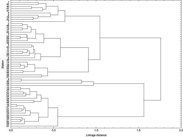
Fig. 2 Dendrogram for 59 standardized anomalies of the monthly precipitation through the Zacatecas state territory using the amalgamation rule of the Ward’s method and the distance metric of 1-Pearson’s r.
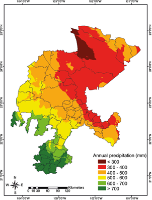
A map showing the stations and their corresponding regions is presented in Fig. 3. Those regions are distributed from NE to SW of the state territory, that is, from the driest to the wettest areas. As expected, cluster analysis results agree with the spatial distribution of the annual mean precipitation throughout the Zacatecas state territory (Fig. 4). Thus, cluster I (semi-arid region) includes weather stations with annual precipitation from < 300 to 400 mm, cluster II (highlands region) includes stations with annual precipitation from 400 to 500 mm, and cluster III (canyons region) includes stations with annual precipitation from 500 to > 700 mm.
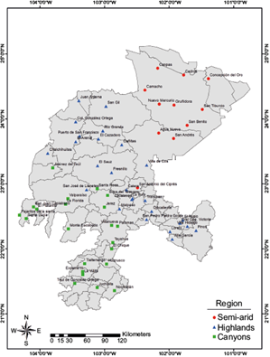
Fig. 3 Location of the weather stations and their corresponding regions found through the cluster analysis in the Zacatecas state territory.
The regions identified in this research agree well with the three floristic districts reported by Balleza et al. (2005) on the basis of the geographic distribution of 456 species of the Asteraceae family. Considering results from both studies, the semi-arid region covers the floristic district named Ia; the Highlands region agrees with the floristic district named Ib; and the canyons region covers the floristic district named II. This implies Asteraceae family species richness and their distribution could depend on the rainfall patterns as suggested by our results. In this context, Balleza et al. (2005) results suggest that the species of the Asteraceae family distributed in the Zacatecas territory can be divided into two main groups: (i) those thriving mostly in the dry environments (semi-arid region), and (ii) those thriving in the temperate, warm habitats along the highlands and canyons regions. In fact, the flowering plant family Asteraceae is one of the most influential in the diversification and evolution of many animals that heavily depend on their inflorescences to survive (Barreda et al., 2015). Species of the Asteraceae family are found almost everywhere in the world except in Antarctica (Barreda et al., 2015), which means that their climatic requirements are very diverse, although it seems that climatic factors restrict the phenological period of most species as pointed out by Torres and Galetto (2011).
Rainfall patterns define the agricultural activities performed by peasants and growers of each region. Such activities represent an important economic income to most of the families settled throughout the Zacatecas territory. In the semi-arid region, goats are kept for dairy and meat production although those activities represent only low income at a family level; the major production systems are characterized by small flocks (< 100 animals), feeding based on grazing and browsing native vegetation, following regular routes and keeping the animals overnight in rudimentary shelters. The main products of these systems are kid goats (“cabritos”) and culled goats (Tovar-Luna, 2009). In the highlands region, the main crop is dry beans (Phaseolus vulgaris), followed by species for forage such as corn (Zea mays) and oats (Avena sativa), and horticultural species such as peppers (Capsicum annum), onions (Allium cepa) and garlic (Allium sativum). In the canyons region, the main activity refers to the cow-calf production system followed by the production of guava (Psidium guajava), and a great variety of horticultural products.
3.2 Power spectrum analysis
A spectral analysis was performed on each regional SAMP series to estimate their self-affinity statistics (Table II): mean, median, standard deviation (Std), fractal dimension (D s ), Hurst exponent (H) and slope (-β). All three regional SAMP series yielded straight lines on the log-log plot with -β, suggesting that P(f) ~ f -b (Valdez-Cepeda et al., 2003a, b). This means that each spectrum is singular and is represented by a curve on the complex plane for the SAMP series of the case.
Table II Basic and fractal statistics for standardized anomalies of the monthly precipitation for the Zacatecas state regions.
| Region | Mean (mm) | Median (mm) | Std (mm) | Ds | H | -β |
| Semi-arid | 29.20 | 20.71 | 29.83 | 1.354 | 0.646 | 2.291 |
| Highlands | 36.07 | 19.82 | 41.75 | 1.497 | 0.503 | 2.007 |
| Canyons | 50.26 | 23.72 | 58.17 | 1.527 | 0.473 | 1.946 |
Note: Std (standard deviation), Ds (fractal dimension), H (Hurst exponent), -β (slope).
Spectral D s values vary from 1.354 to 1.527, and H values change from 0.473 to 0.646. The D s and H values of 1.354 and 0.646, respectively, suggest that the semi-arid region SAMP series tends to show persistent behavior (D s < 1.5 and H > 0.5). The highlands region SAMP series has D s and H values of 1.497 and 0.503, respectively, while the canyons region SAMP series has D s and H values of 1.527 and 0.473, respectively. These results indicate that the SAMP series in both regions tend to be like the Brownian movement or random walk (D s ≈ 1.5), as pointed out by Mandelbrot (1985).
3.3 Important frequencies
Plots of power spectrum density [Φ x (f)] against frequency allow us to identify the dominant frequencies on the regional SAMP series in terms of the dominant frequencies (1 year-1) that are likely to be important to the precipitation process (Fig. 5a-c). This approach gives us some frequency components that do not consider time and length because the analysis gives us a resolution in a frequency that is determined for the window size over the analyzed time series. In other words, the results give us useful information about the frequency content of the analyzed series, but they do not indicate at which time these frequencies occur. The detected frequencies were those from confidence bands of 95% in the adjusted linear model and are likely to be important to the precipitation process. Significant peaks of the power spectrum were detected at p ≤ 0.05.
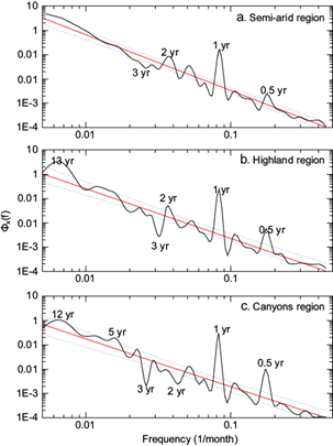
Fig. 5 Power spectrum plots of the monthly mean standardized anomalies of the monthly precipitation time series for (a) semi-arid region, (b) highlands region and (c) canyons region of Zacatecas, Mexico from January 1976 to December 2010, showing important frequencies in years. The power spectral density is given as a function of frequency for time scales of 2 to 408 months. The fitted line was used to estimate the fractal dimension (Ds). Dashed lines indicate the confidence interval at p ≤ 0.05.
The 0.5-, 1-, 2- and 3-year frequencies are present in the power spectrums of all analyzed regional SAMP series. The highlands and canyons regions showed important frequencies of 13 and 12 years, respectively.
The 0.5- and 1-year frequencies may be linked to the seasonal cycle while the 2-year frequency could be related to the Quasi-Biennial Oscillation (Kane, 2009), which is a 26-month cycle explaining solar activity and wind reversal in the lower stratosphere of the North Pole (Labitzke and Loon, 1989; Mendoza et al., 2001). The 3-year frequency suggests a possible effect of a quasi-periodic event like ENSO. It is widely recognized that ENSO has an erratic cycle from 3 to 5 years (Weber and Talkner, 2001), 3 to 6 years (Monetti et al., 2003), 4.3 years (Luo et al., 2015), or 2 to 7 years (Zubair, 2002; MacMynowski and Tziperman, 2008). These discrepancies may be explained by the physical dependence of ENSO frequency on the structure of the coupled mode provided by diagnosing the relative contributions of the thermocline feedback and zonal advection feedback on ENSO evolution (An and Wang, 2000). The 12- and 13-year frequencies indicate that there may be effects from the sunspot cycle, which varies from 8 to 14 years (Mendoza et al., 2001) or 11 years (Hu et al., 2009) with a long-term average of 11.3 years. We then carried out a wavelet coherence analysis on each of the SAMP and the MEI time series, each with a significant 5.5-year frequency, to identify possible relationships.
3.4 Wavelet coherence analysis
Results of phase and wavelet coherence between each regional SAMP series and the Multivariate ENSO Index series are shown in Figure 6a, b, and c, which correspond to the semi-arid, highlands and canyons regions, respectively. The black figure outlines indicate areas significant to 95% confidence, that is, cones of influence; spots limited by a thick black line point out a possibly significant relation between both phenomena; and vectors indicate the phase difference between the regional SAMP and the MEI series with arrows pointing clockwise to indicate in-phase behavior and arrows pointing counter-clockwise to indicate anti-phase behavior (Keener et al., 2010).
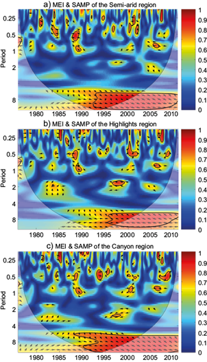
Fig. 6 Wavelet coherence and phase between standardized anomalies of the monthly precipitation (SAMP) of (a) semi-arid region, (b) highlands region, and (c) canyons region (c), and the Multivariate ENSO Index (MEI) for the Zacatecas state. Vectors indicate the phase difference between the SAMP and MEI. Thick black figure outlines indicate areas significant at a 95% confidence level using the red noise model, and the thin black line surrounds the cone of influence.
3.4.1 Semi-arid region
A significant spot is clearly noted from 1993 to 2003 at 5 to 12-year periodicities (Fig. 6a), indicating a high correlation between the semi-arid SAMP and the MEI. It should be highlighted that 1997 was a year of El Niño at very strong intensity, whereas 2002 and 2003 were years of El Niño at moderate intensity (Wolter and Timlin, 2011); 1995, 1996, 2000 and 2001 were years of La Niña at weak intensity (Wolter and Timlin, 2011). The MEI may have been related to precipitation in this semi-arid region during those years. The MEI and SAMP were in phase from 1993 to 2003 as indicated by the horizontal arrows, meaning that the relative phase lag between those phenomena was nil.
Important areas are identified from 1983-1985, 1988-1990, 1996-1997, 2000-2001, and 2002-2003 in the 0.5-year period. These results suggest that seasonal components of the precipitation are important issues in this region. In fact, heavy unimodal precipitation dominates throughout the Zacatecas territory. Significant spots are also identified from 1989-1990 and 2005-2006 at the 1-year period and as such, the precipitation of those years could be related to the movement of the Earth around the sun. The significant spot from 2005 to 2006 corresponds to a period with ENSO and precipitation in phase and SAMP were positive, indicating a humid period.
3.4.2 Highlands region
A significant band of 5- to 12-years is also localized from 1995 to 2003 at 5- to 12-year periodicities (Fig. 6b). Arrows suggest that the highlands region SAMP and the MEI were mostly in phase during this period. This also implies a strong correlation between the MEI and the highlands region SAMP. It is widely recognized that periodicities of El Niño and La Niña are 2-5 and 7-15 years, respectively, as pointed out by Wolter and Timlin (2011). El Niño occurred at moderate intensity from 2002 to 2003, and La Niña events were recorded from 1998 to 2000 at moderate intensity as well.
A significant spot is present from 1996 to 1999 at a 2-year period and another significant small blob is appreciated in 1983, thus implying that the MEI and highlands region SAMP corresponding to these years were strongly correlated. Both phenomena were in anti-phase during 1996-1999, as indicated by horizontal left arrows, which may be explained by the El Niño phenomenon with very strong intensity that occurred during 1997-1998. However, precipitation leads MEI by approximately 1/4 cycle, as indicated by vertical arrows, in 1983. This implies that precipitation during that year could have adhered to El Niño with very strong intensity, which occurred during 1982-1983.
Significant spots occur over 1984-1985, 1986-1988, 1994-1996, 2000-2002, and 2008-2009 at a 0.5-year period. These results suggest that seasonal components of precipitation are important issues in the highlands region. Significant spots are also appreciated over 1989-1990 and 2000-2001 at a 1-year period. Precipitation during these years could therefore be related to the rotation of the Earth around the sun.
3.4.3 Canyons region
A large significant spot is present from 1988 to 2003 at 5- to 10-year periods (Fig. 6c). This result suggests a strong correlation between the MEI and the canyons region SAMP that could be due to periodicities of El Niño and La Niña of 2-5 and 7-15 years, respectively (Wolter and Timlin, 2011). Vectors indicate that the MEI and the SAMP are mostly in phase. In addition, a significant spot present over 1996-1998 at the 3-year period may suggest a strong correlation between the MEI and the canyons SAMP. Both phenomena of the blob were in anti-phase and this could be due to the fact that 1997-1998 was a period of El Niño with strong intensity and 1998-1999 was a period of La Niña with moderate intensity.
Significant spots occur over 1984, 1988-1989, 1993-1994, 2001, and 2006-2009 at a 0.5-year period. These results suggest that seasonal components of precipitation have an important influence in this region. Another important spot was present for the period of 1988-1989 at the 1-year period. As previously stated, precipitation during these years might have been influenced by the Earth’s orbit around the sun.
In summary, we obtained compelling evidence of important spots corresponding to 2- to 7-year periods as shown in the wavelet coherence figures. The significant spots recorded from 1993 to 2003, 1995 to 2003, and 1988 to 2003 for the semi-arid, highlands and canyons regions, respectively, indicate that SAMP vary by region and over time. These results suggest important correlations between the MEI and each of the regional SAMP for the state of Zacatecas. This correlation has also been recorded in other regions around the world such as the precipitation anomaly time series registered at the Litter River Watershed, Tifton, GA, USA and the ENSO 3.4 (Keener et al., 2010).
4. Conclusions
A cluster analysis was successfully performed on 59 SAMP series to identify three regions: semi-arid, highlands and canyons. These regions strongly agree with three floristic districts previously reported and results from both studies suggest that species richness of the Asteraceae family could depend on regional precipitation regimes. These regions agree with areas under the basis of annual mean precipitation in the state of Zacatecas.
Cross correlations using wavelet coherence analysis between the MEI and each of the three regional SAMP series indicate teleconnections at different periods. In the semi-arid region, a strong correlation from 1993 to 2003 occurred between the MEI and SAMP at a 5-12-year period showing a consistent in phase angle. In the case of the highlands region, the results are compelling evidence regarding the influence of ENSO on precipitation. An important correlation from 1995 to 2003 occurred between both phenomena in-phase at a 5-12-year period. Another strong correlation from 1996 to 1999 with an important anti-phase angle was identified and these phenomena were strongly correlated at a delay of approximately 1/4 cycle during 1983. This knowledge could be useful to policymakers since horticultural systems are performed under irrigated conditions using extracted water from aquifers without recharging. The years when El Niño occurs, implying wet seasons, could thus be used to recharge aquifers in this region. In the canyons region, the identified relationship between both phenomena was in phase from 1988 to 2003 and another strong correlation showing antiphase status was found from 1996-1998. There is still a need to measure the degree of association between precipitation and the MEI at regional and local levels by means of other robust statistical techniques, e.g., cross-correlation coefficients, focusing on periods lower than 1 year.
Other identified significant frequencies, i.e., 12 and 13 years for canyons and highlands regional SAMP (Fig. 5), respectively, indicate that their underlying relationships to physical mechanisms remain unknown. In future work, therefore, a wavelet coherence analysis between a quasi-periodic phenomenon (e.g., solar activity measured through the sunspot number time series) and the regional or local SAMP series should be performed to learn more about precipitation behavior.

