


Servicios Personalizados
Revista
Articulo
 Inglés (pdf)
 Artículo en XML
 Referencias del artículo
 Enviar artículo por email
Indicadores
-
 Citado por SciELO
 -
 Accesos
Links relacionados
-
 Similares en
SciELO
Similares en
SciELO
Compartir

 Permalink
Atmósfera
versión impresa ISSN 0187-6236
Atmósfera vol.23 no.3 Ciudad de México ene. 2010
Atmospheric boundary layer height calculation in México City derived by applying the individual eulerian box model
O. ZELAYA–ÁNGEL, S. A. TOMÁS, F. SÁNCHEZ–SINENCIO
Departamento de Física, Centro de Investigación y de Estudios Avanzados, Instituto Politécnico Nacional, Av. IPN 2508, México 07360 D.F., México
V. ALTUZAR, C. MENDOZA–BARRERA
Centro de Investigación en Micro y Nanotecnología, Universidad Veracruzana, Av. Ruiz Cortines 455, Boca del Río 94294, Veracruz, México.Corresponding author: V. Altuzar; e–mail: valtuzar@uv.mx
J. L. ARRIAGA
Laboratorio de Química de la Atmósfera, Instituto Mexicano del Petróleo, Eje Central Lázaro Cárdenas 152, México 07730 DF, México
Received June 6, 2009; Accepted March 23, 2010
RESUMEN
Las emisiones de etileno son características de las exhalaciones primarias de los procesos de combustión vehicular. Su reacción con radicales hidroxilo en presencia de radiación solar UV promueve la producción de ozono. En investigaciones anteriores nuestro grupo reportó la medición de los perfiles en tiempo real de la concentración de etileno en la atmósfera de la Zona Metropolitana de la Ciudad de México mediante un sistema láser fotoacústico de 12C16O2. En este trabajo, aplicamos el modelo fotoquímico de la caja de Euler para ajustar las curvas de concentración de etileno experimental dependientes del tiempo registradas en la semana laborable del 19 al 23 de febrero de 2001. Ello permitió calcular la variación continua de la altura de la capa de mezcla (HABL) comprendida entre las 5:00 y las 21:00 h, en condiciones atmosféricas estables. De dicho perfil, se determinaron las correspondientes curvas temporales de HABL para toda la semana de campaña y el perfil general, de tres picos máximos, de la razón de emisión de etileno por unidad de área q(t). El rango de valores de la altura de la capa de mezcla inicial, por la mañana, osciló entre 169 y 357 m; mientras que por la tarde fue entre 2700 y 3869 m. El modelo de Euler aplicado bajo estas condiciones predice corrimientos de los tres picos máximos en función de las horas de mayor tráfico en la caja de Euler.
ABSTRACT
Ethylene emissions are characteristic of primary exhalations of vehicular combustion processes. Their reaction with hydroxyl radicals in the presence of solar UV radiation promotes the production of ozone. Previously, our research group reported the measurement of real–time profiles of ethylene concentration (EC) in the atmosphere of the Metropolitan Zone of México City (MZMC) by means of laser photoacoustic system, based on 12C16O2. In this work, we applied the Euler box photochemical model to fit the time–dependent experimental ethylene concentration profiles recorded in the working week February 19–23, 2001. Those profiles allowed us to calculate the continuous variation of the atmospheric boundary layer (HABL) between 5:00 and 21:00 h, under stable atmospheric conditions. From the fitting function C(t), we identified the corresponding HABL temporal curves for the entire week of the campaign. Also, the emission ethylene rate general profile q(t) was determined, presenting three maximum peaks. The values of the HABL height ranged between 169 and 357 m in the morning and between 2700 and 3869 m in the afternoon. The Euler model, applied under atmospheric stable conditions, predicts the shifts of the three q(t) maximum center peaks depending on rush hours, Euler box volume, and –OH and ethene reactions.
Keywords: Ethene, ethylene, photoacoustic, pollution, atmospheric boundary layer.
1. Introduction
The region of the atmosphere which governs the vertical and horizontal exchanges and the dispersion of pollutants is called the mixed layer or the atmospheric boundary layer (ABL). It is in this layer where all the primary pollutants coming from vehicular combustion and industrial processes are located. Generally, in a typical day in México City, the ABL height (HABL) growths range from approximately 300 m in the early morning hours to 4000 m in the early afternoon (Doran et al., 2007, 1998; Fast and Zhong, 1998; Raga et al., 1999). The meteorological data are important for understanding the transport and dispersion of pollutants within an airshed and across its boundaries. In general, the parameters measured are: the wind speed and direction, atmospheric pressure, solar radiation, humidity, temperature, and finally HABL. The quantitative measure of the transport and dispersion of air pollution into the atmosphere is indispensable for developing atmospheric chemical transport models that provide information about the individual atmospheric processes and their interactions (Shaw et al., 2007).
The eulerian box (EB) approach is widely used in air pollution modeling (Zlatev, 1989; Fay et al., 1995; Sportisse, 2001; Ortega et al., 2004). Ortega and co–workers have successfully used the model to predict the ozone concentration profiles in the city of Barcelona. On the other hand, Zlatev calculated the profile of several anthropogenic emissions in some cities of Denmark from 1989 to 1998; these calculations were consistent with the measured data. These results show the importance of the EB model to predict the behavior of pollutant emissions in the coming days, by supposing other known environmental parameters. Fay and co–workers carried out several experiments by releasing inert gaseous samples in several ground–level sampling sites in North America, which were detected after 24 hours. The agreement between the EB model prediction and the measured values opens the possibility to simulate the transport of contaminants along relative long distances. In México City, the EB model was used with good results by Young et al. (1997) to measure NOx and O3 concentrations in the atmosphere.
The aim of this work is to establish a relatively simple procedure to calculate the HABL in stable conditions from the measurement of concentration profiles of pollutants in the atmosphere, in particular in the Metropolitan Zone of México City (MZMC). In our case, we have carried out minute–measurements of the ethene concentration (EC) emitted from 5:00 to 21:00 h in the atmosphere of the MZMC from February 19–23, 2001. The experiments were performed by using a CO2 laser–based photoacoustic system, mounted at ground level (Altuzar et al., 2003, 2005). The experimental data together with the EB model allows the calculation of the HABL versus time behavior in the same interval of time, covering mostly the period of motor vehicle traffic circulation in México City. The EB model successfully calculated the ethene profiles during the weekday study, and also predicted the maximum mass emission rate peak qi with time, assuming always the same number of vehicles circulating. The determination of the continuous variation of the ABL height in stable conditions from relatively simple measurements of EC added to the knowledge of meteorological data can be used to predict this HABL in the future in MZMC. HABL can be predicted by considering stable atmospheric conditions and forecasting other weather parameters including average temperature, wind speed, etc. This approach can also be extended to various other cities in the world.
2. Theory
2.1 The eulerian box model
The eulerian individual box model is the simplest among all the photochemical models. It is based on the mass conservation equations of the gaseous species inside a fixed Eulerian box volume. If the dimensions of the box are HABL = H the height and ΔxΔy the area, the equation of the mass balance for the Ci concentrations, where i represents a specific pollutant, has the following form (Seinfeld, 1998) for the zero–dimensional case (the wind speed along the x–axis):
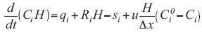

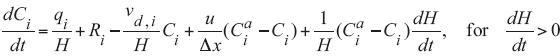
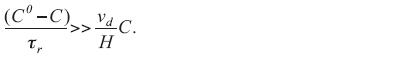
where qi is the mass emission rate of "i"(kg m–2h–1), Ri is the chemical production rate (kg m–3 h–1), si is its removal rate per unit area (kg m–2 h–1), Ci0 represents the background concentration (kg m–3), u is the wind speed (m s–1) (which will be assumed to have a constant direction), and si = vd,iCi, where vd,i describs the dry deposition velocity of the species. The residence time  of the air on the ΔxΔy area is defined as the ratio of the length of the box (Δx) to the prevailing wind speed u: = Δx/u. In the case when H(t) increases and the concentration aloft the box is Ciª, the Eq. 1 is reduced to:

2.2 The ABL height in stable conditions
Figure 1 depicts the temporal profiles of the ABL height calculated from meteorological data and particle dispersion model by Fast and Zhong in México City between 5:00 to 21:00 h on March 4, 1997, within a four–week field campaign. The curve has, until certain limits, a universal form for HABL  H(t) in stable atmospheric conditions, as can be observed in H(t) versus t line shape reported in literature (Seibert et al., 1997; Khandwalla et al., 2002; Margulis and Entekhabi, 2004; Gryning, 2005). In order to fit the H experimental data, we used a Boltzmann function:
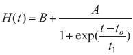

where B represents the afternoon value of ABL height, A is the subtraction between the early morning and the late afternoon ABL height values, t1 is the curve width, and t0 is the curve center. Figure 1 shows a good fit (R2 = 0.99022) of Boltzmann function with the curve of experimental Fast–Zhong data, with B = 2761 m, A = –2533 m, t1 = 0.70 h, and t0 = 13.13 h.
3. Experimental
The photoacoustic (PA) effect is based upon the conversion of electromagnetic energy into acoustic energy (Sigrist, 1994; Harren and Reuss, 1997). A system that is excited by the absorption of light and that undergoes subsequent non–radiative de–excitation processes transfers its electronic, vibrational, and/or rotational energy into translational energy, producing a temperature increase. When the absorption is modulated, the temperature changes periodically, leading to pressure (acoustic) oscillations that can be detected by a sensitive microphone. The PA spectrometer used in this work (Altuzar et al., 2003, 2005) consists of a continuous wave 12C16O2 laser and a PA trace gas detection system. The laser wavelength can be tuned at around 80 lines in the 9 to 11 µm infrared region. The intracavity laser power typically reaches 40 W at the lines selected for measurements. The PA cell is placed inside the cavity of the laser and is designed as a cylindrical acoustic resonator, extended by two buffer volumes, to amplify the generated sound wave due to absorption. The volume of the acoustic resonator is 4.24 cm3, which implies that the resonator has an air–exchange rate of 3.8 s when using a flow rate of 4 liters/hour. The laser beam is intensity–modulated by means of a mechanical chopper locked at the resonance frequency of the PA cell (1160 Hz). The PA system was calibrated using a certified gas mixture of ethene buffered in air (1.2 ppmV ethene). The PA signal is recorded by means of an electret microphone connected to a lock–in amplifier.
The most general situation in PA gas detection involves the measurement of multicomponent samples. PA signals, normalized with the laser power to account for power fluctuations, have therefore to be measured on several laser lines coinciding with absorption bands of the compounds under study. A subsequent least–squares analysis (Bernegger and Sigrist, 1990) provides the concentration of the different gases constituting the mixture. In the present work, we have restricted ourselves to the detection of ethene. The 10P14 (λ = 949.48 cm–1) and 10P12 (λ = 951.19 cm–1) laser lines were selected to determine the ethene concentration in the surrounding air. At these lines, the optical absorption coefficients for ethene were 30.4 and 4.31 cm–1 atm–1, respectively. The recording of the PA phase was not important because CO2 and water vapor were eliminated from the airflow by inserting KOH and CaCl2 scrubbers in combination with a cold trap (Moeckli et al., 1998). To avoid additional problems, Teflon tubing was used. The time resolution was mainly imposed by the time needed to position the grating on the selected laser lines. It resulted in nearly 1 minute. The detection limit for ethene was 100 pptV, as determined from a signal–to–noise ratio equal to one when the PA cell is operated in a continuous–flow mode. Estimating an average uncertainty of 3% for the cell constant, 2% for the certified gas concentration, 1% for 4 liters/hour flux of molecules transported through PA cell, and 1% of random error of the measurement, one finds an overall uncertainty for PAS data of about 7%.
4. Results and discussion
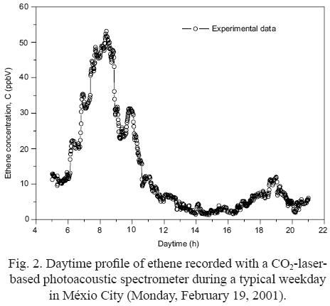
Real–time monitoring of ethene was carried out at the facilities of the Departamento de Física, Centro de Investigación y Estudios Avanzados, Instituto Politécnico Nacional (CINVESTAV–IPN). Ambient (outdoor) air was continuously pumped to the photoacoustic spectrometer from 5:00 to 21:00 h during weekday, from February 19–23, 2001. Figure 2 shows the typical weekday experimental ethene concentration profile versus the daytime plot registered by the PA system on February 19, 2001 (Monday).
For ethene (EC C), Eq. 2 can be written as


Here R = –kC, where k is the rate constant. The ethene molecule is very reactive in presence of hydroxyl radicals (–OH). The value k = 0.7 days–1 (Atkinson and Arey, 2003) will be taken for an average OH concentration of 8.52 x 107 cm–3, which are typical values in large cities (Atkinson and Arey, 2003; Shirley et al., 2006). From the measured profile we found that C0 = 2.44 mg/m3. The average wind speed was close to 1.0 m/s during the week–long study. In the case of the main anthropogenic emissions, above the box Ci = 0, and then Ca = 0. We will assume that our box has an area of 25 km2 and the total area of the MZMC is around 2500 km2. This data determines the value of if we take into account that:

Then, Eq. 4 reduces to:
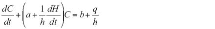

where a = k + 1/and b = Co/. In Eq. 6, to calculate the mass emission rate q(t), we used the ethene experimental data C(t) measured on Monday, February 19 (Fig. 2) and the corresponding Boltzmann fitting H(t) function (Fig. 1). This arrangement is done only to know the general form of the q(t) function. The line shape of this function is showed in Figure 3.
The q(t) function was fitted by using three Lorentzian curves, and the resulting equation is:
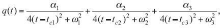

where αi=2aiωi/π (i = 1, 2, 3), ai is the total area under the curve from the baseline, ωi is the full width of the peak at half height, and tciisthe center of the peak. The resulting q(t) fitting parameters are: α1 = 40914.77 µg x h/m2, α2 = 27891.67 µg x h/m2, α3 = 80886.93 µg x h/m2, ω1 = 1.76 h, ω2 = 2.21 h, ω3 = 1.81 h,tc1 = 7.42 h, tc2 = 13.01 h, and tc3 = 18.17 h. By substituting q(t) (Eq. 7) and H(t) (Eq. 3) in Eq. 6, and carrying out the integration process we get to the analytical relation of C(t):
where 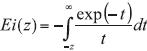 is the exponential integral (Abramowitz and Stegun, 1972).
In order to fit the experimental ethene concentration C(t), we applied Eq. 8. The A, B, t0, t1, tc1, tc2, tc3, and d parameters values were determined by using the least square fitting. The d values were determined by the initial condition of the experimental ethene concentration C(t = 5h) of each day. On the other hand, the ai and ωi parameters were fixed, meaning we supposed the same mass emission rate q(t) of ethene on each day because we assumed that we had the same amount of motor vehicles circulating inside the EB box volume throughout the weekday campaign.
Table I summarized all the C(t) parameters values and the initial ethene concentration C(t = 5 h). We selected the best parameter corresponding to the minimum root mean square error (MRSE) after running 1.5 x 10⁶ iterations (Nvidia Tesla workstation).
It is observed that the EB model predicts the shifts of the center peaks tci(i = 1, 2, 3) of q(t). (See Figure 3). Those shifts are due to their dependence with vehicle traffic, EB volume, and –OH and ethene reactions. In fact, because C(t) is changing with day time, the q peak shifts are the result of rush hours. In addition, we included the A, B, t0 parameters corresponding to H(t) function. Finally, by taking C at 5:00 h we calculated the integration constant d for each day of the campaign.
Figure 4 depicts the experimental and theoretical C(t) profiles obtained for the weekday campaign (Wednesday and Friday are not shown). The result of the fitting has been included in the figure as a solid continuous line. We observed that the data and the fitting are in complete agreement (MRSE ranged from 91.43 on Monday to 150.98 on Thursday).
Figure 5 shows the time evolution of the ABL height for weekdays from March 19–23, 2001 by applying the EB model approach. Hi corresponds to the initial value of H(t) at 5:00 h, whereas Hf is the final value at 21:00 h. We observed that H(t) changes during the daytime and also with a particular weekday, as was expected. The highest Hf occurred on Tuesday (3868.99 m) whereas the lowest ABL Hf was on Thursday (2699.99 m). On the other hand, the maximum value of Hi was of 357.01 m for Friday and the minimum was 169.00 m for Tuesday.
5. Conclusion
In this work we have proposed a relatively simple method to calculate the atmospheric boundary layer height variation as a function of time under stable conditions, in the metropolitan area of México City. Real–time minute–measurements of ethene concentration, registered by means of a CO2–laser based photoacoustic system from 5:00 to 21:00 h, provides the ethene profile. The fitting of the ethene profile with Eulerian Box model and to a general formfor the rate emission function q(t), allows the calculation of the numerical parameters that are involved in the H(t) function.
Acknowledgments
This work was partially supported by the Instituto Mexicano del Petróleo through project IMP–FIES–97–07–VI and by CONACyT through the project 33126–E. The authors thank the RAMA authorities for allowing the use of their database, and Sergio Mendoza (Global Labs. México) for his technical support during the Matlab iteration modeling.
References
Abramowitz M. and I. A. Stegun, 1972. Handbook of mathematical functions: with formulas, graphs, and mathematical tables. NY. Dover Publications Inc. 1047 pp. [ Links ]
Altuzar V., S. A. Tomás, O. Zelaya–Angel, F. Sánchez–Sinencio and J. L. Arriaga, 2003. Atmospheric pollution profiles in México City in two different seasons. Rev. Sci. Instrum. 74, 501–503. [ Links ]
Altuzar V., S. A. Tomás, F. Sánchez–Sinencio, J. L. Arriaga, O. Zelaya–Angel, 2005. Atmospheric ethene concentrations in México City: Indications of strong diurnal and seasonal dependences. Atmos. Environ. 39, 5219–5225. [ Links ]
Atkinson R. and J. Arey, 2003. Atmospheric degradation of volatile organic compounds. Chem. Rev. 103, 4605–4638. [ Links ]
Bernegger S. and M. W. Sigrist, 1990. CO–laser photoacoustic spectroscopy of gases and vapors for trace gas analysis. Infrared Physics. 30, 375–429. [ Links ]
Doran J. C., S. J. Abbott, X. Archuleta, J. Bian, R. L. Chow, R. L. Coulter, S. F. J. de Wekker, S. Edgerton, S. Elliot, A. Fernández, J. D. Fast, J. M. Hubbe, C. King, D. Langley, J. Leach, J. T. Martin, D. Martínez, J. L. Martínez, G. Mercado, V. Mora, M. Mulhearn, J. L. Pena, R. Petty, W. Porch, C. Rusell, R. Salas, J. D. Shannon, W. J. Shaw, G. Sosa, L. Tellier, B. Templeman, J. G. Watson, R. White, C. D. Whiteman and D. Wolfe, 1998. The IMADA–AVER boundary layer experiment in the México City area. B. Amer. Meteorol. Soc. 79, 2497–2508. [ Links ]
Doran J. C., J. C. Barnard, W. P. Arnott, R. Cary, R. Coulter, J. D. Fast, E. I. Kassianov, L. Kleinman, N. S. Laulainen, T. Martin, G. Paredes–Miranda, M. S. Pekour, W. J. Shaw, D. F. Smith, S. R. Springston, and X. Y. Yu1, 2007. The T1–T2 study: evolution of aerosol properties downwind of México City. Atmos. Chem. Phys. 7, 1585–1598. [ Links ]
Fast J. D. and S. Y. Zhong, 1998. Meteorological factors associated with inhomogeneous ozone concentrations within the México City basin. J. Geophys. Res. Atmos. 103, 18927–18946. [ Links ]
Fay B., H. Glaab, I. Jacobsen and R. Schrodin, 1995. Evaluation of Eulerian and Lagrangian atmospheric transport models at the Deutscher Wetterdients using anatex surface tracer data. Atmos. Environ. 29, 2485–2497. [ Links ]
Gryning S. E., 2005. The height of the atmospheric boundary layer during unstable conditions. PhD thesis, Københavns Universitet. Denmark, 64 pp. [ Links ]
Harren F. J. M. and J. Reuss, 1997. Photoacoustic specroscopy. In: Encyclopedia of applied physics. (G. L. Trigg, Ed.). VCH, Weinheim, 19, 413–435. [ Links ]
Khandwalla A., N. Majurec, S. M. Sekelsky, C. R. Williams and K. S. Gage, 2002. Characterization of radar boundary layer data collected during the 2001 multi–frequency radar IOP. Twelfth ARM Science Team Meeting Proceedings. San Petersburgo, Florida. 8–12, April, 1–5. [ Links ]
Margulis S. A. and D. Entekhabi, 2004. Boundary–layer entrainment estimation through assimilation of radiosonde and micrometeorological data into a model–layer model. Bound–Lay. Meteorol. 110, 405–433. [ Links ]
Moeckli M. A., C. Hibes and M. W. Sigrist, 1998. Photoacoustic multicomponent gas analysis using a Levenberger–Marquardt fitting algorithm. Appl. Phys. B 67, 449–458. [ Links ]
Ortega S., M. R. Soler, J. Benetto and D. Pino, 2004. Evaluation of two ozone air quality modelling systems. Atmos. Chem. Phys. 4, 1389–1398. [ Links ]
Raga G. B., D. Baumgardner, G. Kok and I. Rosas, 1999. Some aspects of boundary layer evolution in México City. Atmos. Environ. 33, 5013–5021. [ Links ]
Seibert P., F. Beyrich, S. E. Gryning, S. Joffre, A. Rasmussen and P. Tercier, 1997. Project: Mixing height determination for dispersion modelling. COST Action 710, Preprocessing of meteorological data for dispersion modeling Institute of Meteorology and Physics, University of Agricultural Sciences, Viena, Austria, 120 pp.. [ Links ]
Seinfeld J. H., 1998. Atmospheric chemistry and physics: From air pollution to climate change. John Wiley and Sons, Inc., NY, 880–899. [ Links ]
Shaw W. J., M. S. Pekour, R. L. Coulter, T. J. Martin, and J. T. Walters, 2007. The daytime mixing layer observed by radiosonde, profiler, and lidar during MILAGRO. Atmos. Chem. Phys. Discuss. 7, 15025–15065. [ Links ]
Shirley T. R., W. H. Brune, X. Ren, J. Mao, R. Lesher, B. Cárdenas, R. Volkamer, L. T. Molina, M. J. Molina, B. Lamb, E. Velasco, T. Jobson and M. Alexander, 2006. Atmospheric oxidation in the México City Metropolitan Area (MCMA) during April 2003. Atmos. Chem. Phys. 6, 2753–2765. [ Links ]
Sigrist M. W., 1994. Chemical analysis. In: Air monitoring by spectroscopic techniques. (W. W. Sigrist, Ed.). Series Wiley Inc., NY, 127, 163–238. [ Links ]
Sportisse, B., 2001. Box models versus Eulerian models in air pollution modeling. Atmos. Environ. 35, 175–178. [ Links ]
Young A. T., E. A. Betterton and L. Saldívar de Rueda, 1997. Photochemical box model for México City. Atmósfera 10, 161–178. [ Links ]
Zlatev Z., 1989. The Danish Eulerian model. Meeting on the Assessment of the Meteorological Aspects in the Fourth Phase of EMEP (October 27–30, 1989), Report No. 65. Environmental Pollution Monitoring Programme, World Meteorological Organization, Geneva, Switzerland, 1989, 30–38. [ Links ]

