On the structure of atmospheric waves in middle latitudes

 

A. Wiin-Nielsen

The Collstrup Foundation, H. C. Andersens Boulevard 37, 1553 Copenhagen V, Denmark.

 

Received December 13, 2001; accepted September 9, 2002

 

RESUMEN

La investigación que se describe en este artículo se relaciona con la estructura de las ondas atmosféricas en las latitudes medias. La onda típica en la troposfera tiene, de acuerdo con estudios de observación, una diferencia entre el campo térmico y el campo geopotencial, de tal manera que la vaguada y la cresta en el campo de temperatura se localizan al oeste de las curvas correspondientes al campo geopotencial.

Para explicar los hechos observados se hace un desarrollo teórico utilizando la versión lineal de dos niveles del modelo quasi-no-divergente, incluyendo el calentamiento y la disipación. Este modelo contiene la posibilidad de inestabilidad baroclínica para ciertas longitudes de onda para un cizallamiento vertical del viento suficientemente grande. Es necesario, por lo tanto, tratar los casos estables e inestables por separado. Las técnicas aplicadas incluyen la integración numérica para el estado estacionario en los casos estables y el tratamiento detallado de ecuaciones de perturbación en los casos inestables. Se incluye el cálculo de la velocidad vertical para mostrar que estas ondas convierten la energía potencial turbulenta disponible en energía cinética turbulenta.

Las ecuaciones del modelo están simplificadas de manera que las variables dependientes son las variaciones en la dirección zonal y en el tiempo. El modelo permite el cálculo del transporte meridional del calor sensible; pero dada su simplicidad, el transporte meridional de momento queda excluido. La estructura calculada de la onda se corresponde bien con las ondas atmosféricas observadas en las latitudes medias.

 

ABSTRACT

The investigation described in the present paper is concerned with the structure of atmospheric waves in the middle latitudes. The typical wave in the troposphere has, according to observational studies, a difference between the thermal field and the geopotential field in such a way that the trough and the ridge in the temperature field are located to the west of the corresponding curves for the geopotential field.

A theory using a linear version of the two-level, quasi-nondivergent model including heating and dissipation is developed to explain these observed facts. Such a model will contain the possibility of baroclinic instability for certain wavelengths for a sufficiently large vertical windshear. It is thus necessary to treat the stable and the unstable cases separately. The applied techniques include both a numerical integration to steady state in the stable cases and a detailed treatment of the perturbation equations in the unstable case. A calculation of the vertical velocity is included in order to show that these waves convert eddy available potential energy to eddy kinetic energy.

The model equations are simplified in such a way that the independent variables are the variations both in the zonal direction and in time. The model permits a calculation of the meridional transport of sensible heat, but due to its simplicity the meridional transport of momentum is excluded. The calculated structure of the wave is in good agreement with the observed atmospheric waves in middle latitudes.

Key words: atmospheric waves, middle latitudes, thermal and geopotential fields.

 

1. Introduction

The theories dealing with atmospheric waves consist of two parts. Early baroclinic stability investigations have shown that waves with a wavelength of a few thousand kilometers may be unstable for a sufficiently large vertical windshear (Charney, 1947; Phillips, 1951; Thompson, 1961). Very long transient waves may also be weakly unstable provided that the model contains a vertical variation of the static stability parameter (Wiin-Nielsen, 2001). The stationary very long waves seem to be created by the influences on the flow of topography (Charney and Eliassen, 1949) and the heat sources and sinks of the atmosphere (Smagorinsky, 1952).

The structure of the baroclinic unstable atmospheric waves may be calculated from the results of a stability analysis as done for example by Thompson (1961), Wiin-Nielsen (1989a, 1989b) and Wiin-Nielsen and Marshall (1990). The structure of the waves will be treated in a more elementary way in the present paper.

The purpose of this investigation is to determine the structure of baroclinic waves for various wavelengths, including stable and unstable waves, and thus provide a more detailed and more simple investigation than those presently available in the meteorological literature. To obtain this goal it has been found that the most instructive way is to perform integrations with respect to time of a simple model paying attention to both heating and dissipation. The treatment is thus more general and at the same time more simple than that in earlier studies.

 

2. The basic problem

It is known from the many studies of the baroclinic stability problem in the quasi-nondivergent case that the very long waves are stable for the thermal zonal winds observed in the atmosphere. The waves are generated by the forcing due to the atmospheric heating and the topography. The purpose of this investigation is to use models which are the simplest possible. We shall include the heating effect and the dissipation. In addition, we shall use a two-level quasi-nondivergent model with pressure p as the vertical variable. The basic equations in linearized form are given below in equation (2.1). The susbscript * refers to the 500 hPa level, while the subscript T refers to a layer with a thickness of 250 hPa. In these equations U_* is the zonal wind at 500 hPa, while U_T is the thermal zonal wind for a layer of 250 hPa.

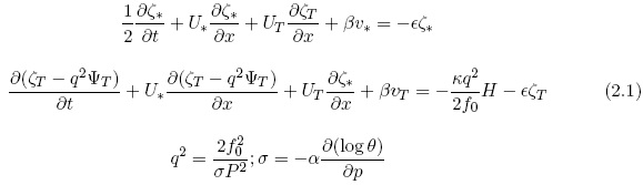
In (2.1), H is the heating and ∈ the frictional coefficient. The vorticity is denoted by ζ, the streamfunction by Ψ, the meridional variation of the Coriolis parameter by β. q² has the dimension m^-2, and contains the static stability parameter σ, which is defined in (2.1). In addition, ƒ₀ is a constant value of the Coriolis parameter, P = 500 hPa, and θ the potential temperature.

Using these equations we shall consider a single wave with wave number k = 2π/L. The variables will, in general, have the form shown in (2.2), where a is an arbitrary dependent variable, while streamfunctions have the special form, also shown in (2.2).

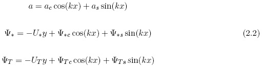
The streamfunction at 500 hPa and the thermal streamfunction for a layer of 250 hPa are the dependent variables in the two equations in (2.1). In addition, we shall be interested in the vertical p-velocity 500 hPa. The basic equations for the standard two-level model can be written in the form given in (2.3) when the specification in (2.2) in introduced.

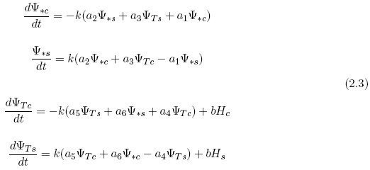
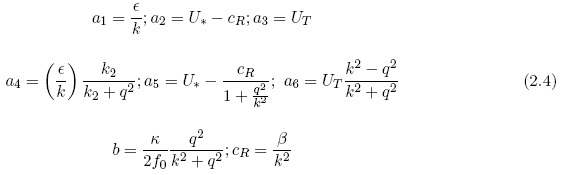
The coefficients appearing in (2.3) have the definitions listed in (2.4).

The equations listed in (2.3) are linear equations for constant values of U_* and U_T. It is necessary to distinguish between two cases. It is well known that the standard two-level model employed in the present investigation results in baroclinic instability for an interval of wavelengths with a sufficiently large value of the thermal wind (U_T). The well known stability diagram is found in Figure 1. It shows instability for a large thermal wind for wavelengths between 4100 km to 28000 km. The minimum value of Ut for instability turns out to be 12.80 m per s. The e-folding times, measured in days and for U_T = 25 m per s are found in Figure 2. The diagrams are computed for q² = 2.5 × 10^-12 m^-2.

In view of the baroclinic instability for some wavelengths it is necessary to divide the investigation in two parts, one for stable cases and another for unstable ones.

 

3. The stable case in the two-level model

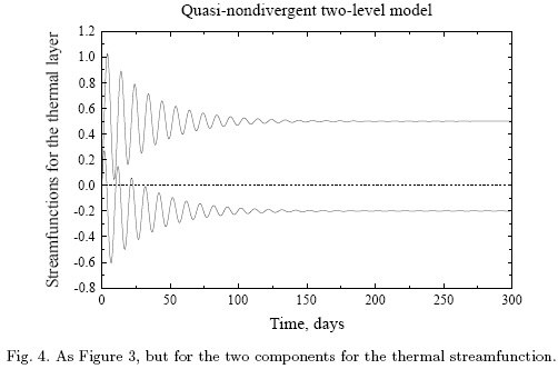
For the stable case we shall investigate a long wave, L = 10 000 km. The heating is set to 3.0 × 10^-3 J/(kg s) for the cosine-component and 1.0 × 10^-3J/(kg s) for the sine component. In addition, U_* = 20 m per s and U_T = 10 m per s in all cases. Using the values chosen for the parameters, we shall determine the four steady state equations, but it is of interest to determine how long it takes to come close to this state starting from a state of rest. Figures 3 and 4 show the time dependence of the four components for an integration over 300 days. They indicate that the steady states are reached with good accuracy after about 200 days. Figure 5 shows the heating for one wavelength.

It is also important to determine the vertical p-velocity. Since we have a steady state it can be calculated either from the thermodynamic equation or from the thermal vorticity equation. The latter equation has been used in the present case.

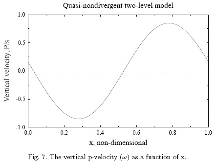
Figure 6 shows the streamfunctions for 500 hPa level and for the thermal layer. The vertical p-velocity is also included in Figure 6 (dotted curve). The three curves have been produced in such a way that the maximum values are one unit to facilitate the comparison between them. It is seen that the thermal streamfunction has its maximum and minimum to the west of the maxima in the streamfunction at 500 hPa in agreement with observations. The two curves for the thermal streamfunction and the vertical p-velocity determine the energy conversion from eddy available potential energy and eddy kinetic energy.

The magnitude of the vertical p-velocity for the present case can be observed in Figure 7, where the maximum value is about 0.8 Pa per s.

The model permits the evaluation of the energy conversion from eddy available potential energy to eddy kinetic energy. In the steady state case we have the relation given in (3.1).

For the present example C(A_E, K_E) = 1.07 W per m². It is also possible to calculate the generation of the eddy available potential energy since we have a specified value of the heating. The result is that G(A_E) = ó0.76 W per m². Since we have additionally made our calculations in a steady state we may conclude that the energy conversion C(A_E, A_E) = 1.83W per m².

 

4. The unstable case in the two-level model

Within the region of instability in the simple, linear, two-level model the strategy applied in Section 3 must be modified to obtain the relations of the waves to one another. If attempted, the growth of the wave amplitude would be observed, and since the zonal flow remains unchanged in the simple model, growth would lead to very large values of the eddy quantities. The solution to the structure problems will in this case be found by using the perturbation equations to obtain the relation between the 500 hPa streamfunction and the thermal streamfunction. After this determination has been obtained we may proceed to calculate the vertical p-velocity and consider its relation to the streamfunctions.

The basic equations are as before the vorticity equations for the 500 hPa level and for the thermal field supplemented by the thermodynamic equation. The two equations for the thermal field are combined to the thermal vorticity equation by the elimination of the vertical p-velocity. As usual the perturbations will have the form shown in (4.1) where a is an arbitrary variable.

It is convenient to recall the curve of the minimum thermal zonal wind necessary to provide baroclinic instability (see Figure 1). The perturbation equations for the model are given in (4.2).

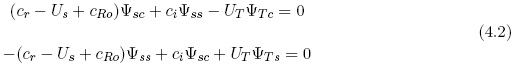
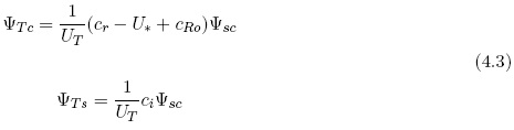
In equation (4.2) the dependent variables are the streamfunction at 500 hPa (subscript ) and the thermal streamfunction (subscript T). The second subscript (c or ) refers to the cosine and the sine components. It will be noted that the two components of the thermal streamfunction can be expressed in terms of the components for the 500 hPa streamfunction. When we furthermore neglect the sine component of the 500 hPa streamfunction we get the result given in (4.3). This procedure is permissible because we are interested in relations between the two streamfunctions.

Having these results it is possible to calculate the phase difference between the two streamfunctions, when the real and the imaginary parts of the phase speed are known. They are given in (4.4).

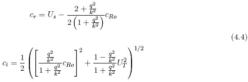
The basic parameters are the same in all the examples, i. e., U = 20 m per s, U_T = 15 m per , q² = 2.5 × 10^-12 m^-2

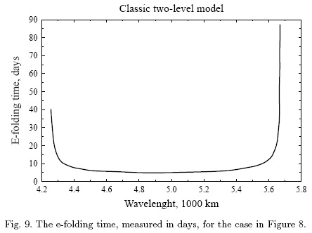
Figure 8 shows the real and the imaginary components of the phase speed in m per s. The upper curve is the real part of the phase speed, while the lower curve gives the imaginary part. It is seen that the wavelength interval goes from about 4250 km to about 5700 km. Compared to the classical case of the phase speeds it will be noticed that the interval is displaced toward longer waves. The reason is that the value of q² has been given the value 2.5 × 10^-12 m^-2 as compared to the commonly used value 4.0 × 10^-12 m^-2. The first value is a more accurate estimate based on observational studies of the static stability and its variation with pressure. Figure 9 contains the e-folding times, measured in days for the unstable wave. The relation between the thermal field (dotted vurve) and the 500 hPa field is seen in Figure 10, where the correct displacement of the thermal field to the west of the streamfunction at 500 hPa is shown.

The vertical p-velocity has also been computed for the example. For this purpose we can use either the thermal vorticity equation or the thermodynamic equation. The result shown in Figure 11 was obtained from the thermal vorticity equation. The result (the dotted curve in Figure 11) is compared with the thermal streamfunction, divided by 1.0 × 10⁷, and the result is the other curve in Figure 11. It is seen that the two curves are almost out of phase indicating that the wave converts eddy available potential energy to eddy kinetic energy.

 

5. The unstable case in the three level model

It is of interest to expand the investigation to models with a higher vertical resolution, because such models may have baroclinic instabilities also for very long waves. To avoid models with very high vertical resolution resulting in cumbersome arithmetic, it was decided to use the three level quasi-nondivergent model with a vertical variation of the static stability parameter. The baroclinic stability in such a model has been studied (Wiin-Nielsen, 1989c), and the results indicate that the vertical variation of the static stability parameter is important, because without this variation very long waves are stable. Based on the earlier baroclinic instability studies it is desirable to expand the analysis to the structure of unstable waves at the three levels.

Perturbation equations for the three levels in the model will be used. The numbers indicating the various levels go from 0 to 6, where 0 is the top of the atmosphere and 6 is the 1000 hPa level. The vertical p-velocities appearing in the model at levels 2 and 4 are eliminated from the vorticity equations by inserting the thermodynamic equations at these levels. The vorticity equation is applied at levels 1, 3, and 5. The thermodynamic equation is applied at levels 2 and 4. At levels 0 and 6 the vertical p-velocities vanish due to the boundary conditions.

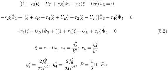
The basic zonal flow is known at levels 1, 3, and 5 with the notations U₁, U₂, and U₃. We also define the two thermal winds U_T = U₁ó U₃, and U_B = U₃ ó U₅. The static stability parameters are σ₂ and σ₄, where the first has a larger value than the second since it is known that the static stability parameter increases as the pressure decreases. It is assumed that the perturbation streamfunctions have the form given in (5.1).

The three equations for the linearized model at levels 1, 3, and 5 are the basic linear equations for the investigation. They take the form shown in (5.2).

The equations in (5.2) are used in the stability investigations from which we determine the real and imaginary values of c for the different wavelengths. This requires that the determinant of the three equations is evaluated leading to a cubic equation in ξ. With regard to the detailed determination of the eigen-values of the three equations as a function fo wavelengths and the main results of the stability analysis reference is made to Wiin-Nielsen (1989c). It will suffice to mention that for the proper values of the two thermal windspeeds, i. e., U_T and U_B, instabilities occur at the wavelengths of a medium size and at the longest waves at the selected latitude (45 degrees North). Figure 12 shows the real values of c as a function of the wavelength. The figure indicates instabilities in an interval of medium long waves and in another interval for very long waves. Figure 13 shows the e-folding times, measured in days, for the shorter waves with U_T = 30 m per s and U_B = 10 m per s. The interval covers a region from below 3000 km to almost 9000 km. Figure 14 shows the same for the very long waves in an interval from 9800 km to 28000 km. It is noted that the strongest instability is at 14000 km, but also that their e-folding times are much larger than for the shorter waves.

The determination of the structure of unstable waves, which is the main purpose of the present paper, is obtained from the equations given in (5.2).

Having the eigen-values as complex numbers for each wavelength we proceed to determine the relative position of the waves. We start by deciding that the wave at 500 hPa shall be described by a cosine function only as shown in (5.3).

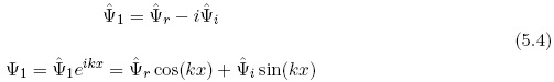
We notice next that the first equation in (5.2) only contains the streamfunctions at level 1 and 3. Knowing the wave at level 3 as seen in (5.3) we proceed to determine the real and the imaginary parts of the streamfunction at level 1. We emphasize that the complex amplitude has to be written in the form shown in (5.4) to obtain the expression for the wave itself in the form also given in (5.4).

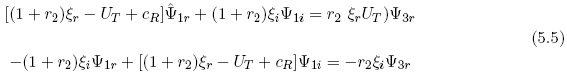
In the first equation in (5.2) we introduce the real and the imaginary parts of the streamfunctions and the wave speed (c). Isolating the real and the imaginary parts of the resulting equations we obtain two equations containing only real values. They are given in (5.5).

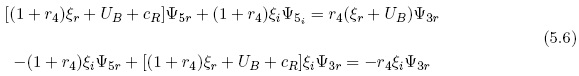
The two linear equations in (5.5) are solved with respect to the two components of the stream-function at level 1. An analogous treatment is used to obtain the real and the imaginary parts of the streamfunction at level 5. The equations are in this case given in (5.6).

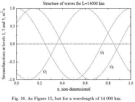
The equations in (5.5) and (5.6) are solved separately giving the real and the imaginary parts of the streamfunction at levels 1 and 5. The waves may then be plotted as shown in Figure 15 for a wavelength of 6000 km and in Figure 16 for a wavelength of 14000 km. Figure 15 clearly shows that the wave slopes toward the west as the pressure decreases, which is the same as saying that the thermal field is lagging behind the streamfunction. A similar result is shown in Figure 16 for a very long wave. It is seen that for the very long wave we obtain a larger separation of the waves at all three levels. Therefore, the major conclusion from experiments conducted so far is that the unstable cases for shorter and longer wavelengths have a similar structure with a slope from east to west with decreasing pressure. We have used wind profiles where U_T > U_B which is typical for the observed zonal winds.

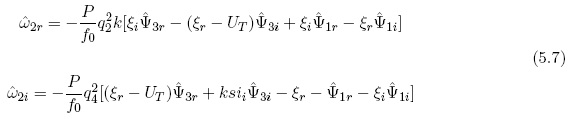
It is also of interest to compute the vertical p-velocities in the model. These can be obtained from the so-called omega equation, from the thermal vorticity equation, or from the thermodynamic equation. It appears that the thermodynamic equation is the most convenient of the three possibilities. In the three-level quasi-nondivergent model we have a vertical velocity at levels 2 and 4. Considering level 2 first, after some calculations we obtain the two components of the vertical p-velocity. The real and imaginary components are given in (5.7).

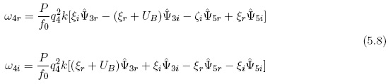
A similar equation for level 4 may be obtained by applying the thermodynamic equation and introducing the zonal flow and the streamfunctions. The result is expressed in (5.8)

Having the amplitudes of the real and imaginary of the vertical velocities at levels 2 and 4 we may finally obtain the curves of the vertical p-velocity. The formulas are given in (5.9).

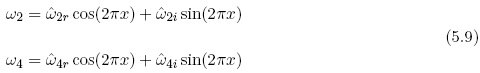
Figure 17 shows the vertical p-velocities at levels 2 and 4 over one wavelength. The values are slightly larger at level 2 (upper troposphere) than at level 4. The two curves are almost in phase with each other. Figure 18 shows the normalized values of the vertical p-velocity and the thermal streamfunction at level 2. The two curves are almost 180 degrees out of phase. As can be seen from Figure 19 a similar situation is present at level 4. With respect to the energetics of the model, both figures indicate that eddy available potential energy is converted into eddy kinetic energy.

 

6. Concluding remarks

The two separate investigations show that both the unstable and the stable waves in a two-level quasi-nondivergent model have a structure in which the thermal field is lagging behind the 500 hPa field. The phase difference in the computed examples varies from 5 to 10 percent of the wavelength.

A similar result is obtained using a three level quasi-nondivergent model. The study of this model indicates a slope from east to west of the unstable waves as pressure decreases. The slope is of the same nature for medium-long waves and for very long waves, but the slope is larger for very long waves.

The calculations of the vertical p-velocity at levels 2 and 4 indicate that the vertical velocities at each level are about 180 degrees out of phase with the thermal streamfunction indicating an energy conversion from the eddy available potential energy to the eddy kinetic energy.

The results obtained in the various cases give a more detailed view of the structure of both medium-long waves than has been obtained in the earlier investigations of the structure of atmospheric waves. The reasons are both the use of models which include the heating and the dissipation and determination of the vertical p-velocity. This study allows us to determine the generation of the eddy available potential energy and the conversion from eddy available potential energy to eddy kinetic energy. In the steady state case it is also possible to determine the conversion of zonal available potential energy to eddy available potential energy.

A Appendix

 

References

Charney, J. G., 1947. The dynamics of long waves in a baroclinic westerly current, Jour. of Meteorology, 4, 135-163.         [ Links ]

Charney J. G. and A. Eliassen, 1949. A numerical method for predicting the perturbations of the middle-latitude westerlies, Tellus, 1, 38-54.         [ Links ]

Philips, N. A., 1951. A simple three-dimensional model for the study of large-scale extratropical flow patterns, Jour. of Meteorology, 8, 381-394.         [ Links ]

Smagorinsky, J., 1952. The dynamical influence of large-scale heat sources and sinks on the quasi-stationary mean motions of the atmosphere, Quart. Jour. of the Royal Meteorological Society, 79, 342-366.         [ Links ]

Thompson, P. D., 1961. Numerical weather analysis and prediction, Macmillan, New York, 170 pp.         [ Links ]

Wiin-Nielsen, A., 1989a. On the structure of transient baroclinic waves, I, Atmosfera, 2, 3-15.         [ Links ]

Wiin-Nielsen, A., 1989b. On the structure of transient baroclinic waves, II, Atmosfera, 2, 189-208.         [ Links ]

Wiin-Nielsen, A., 1989c. A stability investigation of a three-level, quasi-geostrophic model, Geophysica, 25, 21-35.         [ Links ]

Wiin-Nielsen A. and H. Marshall, 1990. On the structure of transient baroclinic waves, III, Atmosfera, 3, 73-109.         [ Links ]

Wiin-Nielsen, A., 2001. On atmospheric waves, to be published by Royal Danish Academy of Sciences and Letters, 50 pp.         [ Links ]