


Servicios Personalizados
Revista
Articulo
 Inglés (pdf)
 Artículo en XML
 Referencias del artículo
 Enviar artículo por email
Indicadores
-
 Citado por SciELO
 -
 Accesos
Links relacionados
-
 Similares en
SciELO
Similares en
SciELO
Compartir

 Permalink
Atmósfera
versión impresa ISSN 0187-6236
Atmósfera vol.15 no.2 Ciudad de México abr. 2002
Seasonal variability of the temperature and heat fluxes in the Gulf of Mexico
J. ZAVALA-HIDALGO,* A. PARÉS-SIERRA and J. OCHOA
*Current affiliation: Center for Ocean-Atmospheric Prediction Studies, Florida State University
División de Oceanología, CICESE, Ensenada, Baja California, México
(Manuscript received, June 6, 2001; accepted in final form Aug. 29, 2001)
RESUMEN
Se estudian los flujos de calor entre la atmósfera y la superficie del mar en el Golfo de México, utilizando los datos climatológicos de la base Comprehensive Ocean-Atmosphere Data Set (COADS), fórmulas empíricas, estimaciones de la radiación mediante satélite y con la ayuda de la modelación numérica. Para los flujos superficiales de calor se obtuvo una media de 9 W m-2. Este valor es más alto que el de estudios previos debido a que se utilizaron distintas fuentes de datos y fórmulas empíricas. Para el ciclo anual se obtuvo una amplitud de 168 W m-2. Se calcula y analiza la contribución de cada término en la ecuación de calor comparando los valores obtenidos con los de estudios previos.
Un modelo numérico con termodinámica es utilizado para estudiar la importancia relativa de la advección de calor y los flujos verticales asociados al aporte de agua de la capa intermedia a la superficial. Los resultados muestran que los flujos entre capas son importantes en el enfriamiento de invierno de las aguas superficiales. Cuando estos flujos, que dependen de la pérdida de flotación y de la inducción de energía cinética turbulenta a través de la superficie, no son incluidos en el modelo, las temperaturas de invierno permanecen nías altas que las observadas y el error cuadrático medio es de 1.5°C, mientras que al incluirlos decrece a 1.0°C.
Palabras clave: Golfo de México, flujos de calor, modelación numérica, temperatura superficial del mar, variación estacional.
ABSTRACT
Heat fluxes between the atmosphere and the sea surface in the Gulf of Mexico are computed using the COADS climatology, bulk formulae, radiation estimations from satellite, and a numerical model. 9 W m-2 is the estimated mean surface heat flux into the ocean, this is higher than previous studies due to different bulk formulae and data sources. The annual cycle has an amplitude of 168 W m-2. The contribution of each term in the heat equation is computed, analyzed and compared to previous studies.
A numerical model with thermodynamics is used to study the relative importance of heat advection and entrainment on the sea surface temperature. The results indicate that the entrainment is important in the winter cooling of surface waters. When entrainment, which depends on the buoyancy loss and the wind induced turbulent kinetic energy, is not included, temperatures in winter stay higher than observations, with a root mean square (RMS) difference from observations of 1.5°C. Including entrainment and detrainment the RMS decreases to 1.0 °C.
Key words: Gulf of Mexico, heat fluxes, numerical model, sea surface temperature, seasonal variability.
1. Introduction
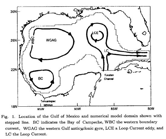
The Gulf of Mexico, a semiclosed marginal sea, is located in the western Atlantic Ocean. It has an area of 1.5 X 10⁶ km2 (Fig. 1) and communicates in the southeastern end with the Caribbean Sea and to the east, through the Florida Strait, with the Atlantic Ocean. Most of the attention in the gulf has focused in its dynamics due to the presence of one of the strongest currents in the world, the Loop Current, which is part of the Gulf Stream current-system. This current sheds large anticyclonic eddies with diameters sometimes larger than 250 km and speeds greater than 1 m s-1, which migrate slowly at about 5 km day-1 to the western gulf (Hurlburt and Thompson, 1980; Elliot, 1982; Vukovich, 1995; Vukovich and Crissman, 1986; Dietrich and Lin, 1994). The wind forcing of the Gulf plays an important role because it drives, or at least reinforces, a western boundary current flowing northward, near the northwestern shelf break of the gulf and the cyclonic circulation in the Bay of Campeche (Sturges et al, 1993; Vázquez, 1993; Zavala et al, 2001).
The gulf also has a high sea surface temperature (SST) variability and an intense seasonal heat flux cycle, which are the main interest of this paper. In the northern part of the gulf, from winter to summer, there is a variation of more than 12°C in the surface waters. The seasonal heat budget of the Gulf of Mexico (GM) has been the subject of several studies which investigated the heat fluxes and modeled the SST (Hastenrath, 1968; Etter, 1983; Etter et al, 1987; Adem et al., 1991; Adem et al, 1993; Adem et al, 1994). Those studies have focused their attention in understanding the changes in one of the so called "heat budgets" of the ocean, defined as 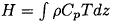 where ρ is the density, Cp is the specific heat and T is the temperature, and the integral ranges from bottom to sea surface. The rate of change of this heat budget is due to the surface fluxes and the advection, as expressed schematically in the relation

where Qs is the net short wave radiation into the ocean, Qb is the heat flux emitted by the ocean as long wave radiation, including cloud feedback, Qe is the heat lost by the ocean due to evaporation, Qh is the heat flux through the ocean-atmosphere interface as sensible heat, and Qa is the horizontal advective heat flux. The left hand side of equation (1) and the term Qa follow directly from the vertical integral of the temperature equation, all other terms are the separation in contributions of the net boundary condition at the upper limit of the integral.
An estimation of δH/δt was done by Etter (1983) using historical hydrographie data. The fluxes due to short-wave and long-wave radiation have been estimated using empirical formulae (Hastenrath, 1968; Etter, 1983; Adem et al., 1993) (hereafter H68, E83, A93). The formulae used by these authors have some differences in their dependence on climatological variables. Turbulent fluxes have been computed in different ways: by bulk formulae (H68, E83, A93), and computing them as a residual using equation (1) (H68). The advected heat has been estimated using the temperature and water fluxes on the Yucatan Channel and the Strait of Florida (H68, E83, A93) or as a residual of the other fluxes using equation (1) (E83).
The vertical heat flux within the water column was estimated by E83 following a method proposed by Emery (1976). This method is based on the vertical variation of the temperature and an equation for the divergence of heat. Adem et al. (1991) worked with a fixed mixed layer of 60 m and concluded that the influence of the vertical fluxes into the mixed layer from below is negligible.
These authors have shown that δH/δt is positive between March and September reaching its maximum in May-June and the minimum in December-January. The sea surface temperature has a maximum in July-August (~29.5 °C) a minimum in February (~17 °C) (values offshore of the continental shelf). The SST is very homogenous in the whole gulf surface during summer while in winter there are strong horizontal gradients. Zavala et al. (1997) show that there are considerable uncertainties on the heat fluxes parameterization.
In spite of the studies mentioned, considerable uncertainty persists in the heat flux estimations. Different proposals of the bulk formulae produce significant differences. The turbulent fluxes, i.e. the latent heat flux, and the sensible heat flux, have been estimated with the same formulae or an equivalent set, but with different value of the turbulent coefficients (Appendix III). In the estimation of the radiation fluxes, different formulae have also been proposed. These fluxes are affected by the presence of clouds whose influence has been considered under different algorithms or values of coefficients, producing odd results. Another source of uncertainty in the estimation of the turbulent fluxes is related to the database used. Some common problems are that not all the regions have enough samples, and some variables have a bias (i. e. ships avoid storms, local influences on costal meteorological data, etc.)
The main interest of this paper is to study the seasonal variation of the surface heat fluxes and the SST in the Gulf of Mexico, with emphasis on understanding the relative importance of advection and entrainment. We analyze in detail the contribution of each term in the heat equation and its influence on the seasonal variability of the SST. The heat fluxes are reviewed computing them by bulk formulae, using radiation data from satellite (Darnell et al., 1992), and numerical modeling. Also, heat fluxes estimated in this work are compared to previous estimations. Data from the Comprehensive Ocean-Atmosphere Data Set (COADS) are considered and a set of bulk formulae are chosen based on the results of recent works by Reed (1983), Geernaert (1990), and Katsaros (1990). The COADS sea surface temperature is also used to qualify model results. Several numerical experiments were done in order to evaluate the importance of different influences on the SST.
In the numerical experiments, a 2½ inhomogeneous layer model (reduce gravity with 2 active layers) is used, similar to those used by McCreary and Kundu, (1988), Schopf and Cane (1983), and McCreary et al. (1993). This model allows for variations, within each of the two active layers, of the horizontal velocity, thickness and temperature, each with dynamic consequences. In particular, the inclusion of laterally varying temperature allows the modeling of non-uniform surface heat fluxes and realistic vertical exchanges between the layers. Forcing mechanisms are the monthly climatological wind stress, the surface heat flux deduced from a Haney's type of equation (Haney, 1971), and prescribed transports for the Yucatan Channel and the Strait of Florida. The entrainment, thickness and temperature of the upper layer follows a Niiler-Kraus mixed layer model.
Section 2 includes a description of the model; sections 3 includes the analysis of the heat fluxes, and section 4 describes the influence on the SST of different terms in the heat equation and the entrainment. Discussion and final remarks are included in section 5. Specifications of the bulk formulae used, a linearization of them, and a compilation of formulae from other works using bulk formulae, are found in Appendices I, II and III, respectively.
2. The Model
A primitive-equations inhomogeneous layered numerical model is used. These kind of models have been used by many authors (Schopf and Cane, 1983; McCreary and Kundu, 1988; McCreary et al, 1993; McCreary and Lu, 1994), the origins of its formulation is not that recent (Dronkers, 1969; Lavoie, 1972). In this study, the model consists of an active upper layer with variable thickness related to the mixed layer, an active intermediate layer, and an infinite depth motionless and homogeneous deep layer. The model allows for the exchange of heat, momentum, and mass through each of the three interfaces. For this work no exchanges are included between the intermediate and deep layers, nor is mass exchanged through the surface. The temperature equations include surface heat flux and cooling due to entrainment from the lower layer. For entrainment it is understood the thickening of the upper layer due to the incorporation of water from the intermediate layer. A mixed layer model was coupled to the upper layer to allow changes of temperature and thickness in the upper layer even in the absence of advection. There is also the possibility of detrainment, the process of thinning the upper layer by expelling a fraction of its water into the intermediate layer. Detrainment does heat up the cooler intermediate layer. The lateral boundaries are either open or vertical walls and the shelf processes as well as its interaction with the interior are not considered in this work. This last feature simplifies to a great extent the numerical model, but it is likely the major limitating factor to be realistic.
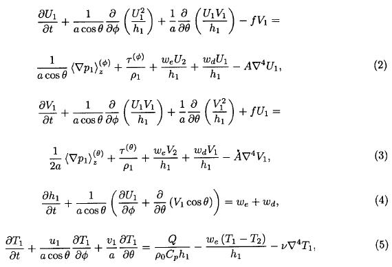
The momentum, continuity, and heat equations for the upper layer are
and for the intermediate layer are
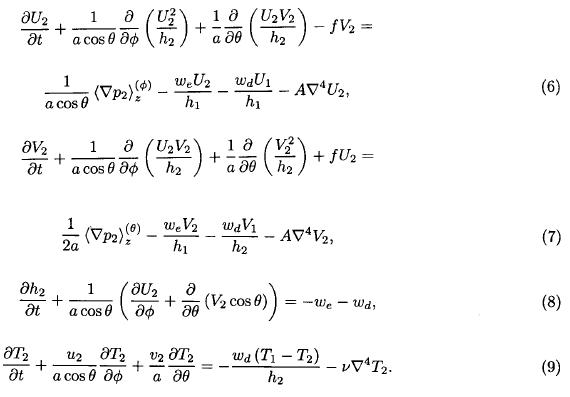
In the above equations, θ is the latitude, Φ is the longitude, ui and vi are the longitudinal and latitudinal components of the velocity respectively, i is the layer index, Ti and hi are the temperature and the layer thickness respectively, Ui ≡ uihi and Vi ≡ vihi, are the transport components, τ(j) is the component of the wind stress in the j direction, Q is the heat flux through the surface, we is the entrainment and wd the detrainment.  is the k component of the depth-averaged horizontal pressure gradient in the layer. A biharmonic damping is used to prevent motions with structure at grid scale while allowing practically undamped large-scale motion (Holland, 1978).
Entrainment is defined as the rate of the upper layer thickness increase due to the influx of water from the intermediate layer and is positive definite. The detrainment is minus the rate of volume water received in the intermediate layer from the upper layer, and is negative definite. The momentum and heat exchanged by the entrainment (detrainment) are distributed uniformly in the vertical on the receiving layer. Notice from the previous equations that total volume (h1 + h2) is conserved.
The depth-averaged pressure gradients are given by
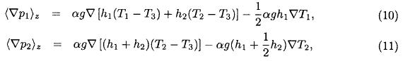
where α is the coefficient of thermal expansion and g is gravity.
The numerical model was run on a C grid (Mesinger and Arakawa, 1976), with a zonal and meridional resolution of 1/6 of degree between the same variable points. A leap frog scheme was used to integrate the equations in time, with a forward derivative every 99 time steps to prevent time-splitting instability. The time step was 20 min. The parameters used in the model are listed in Table 1.

2.1. Forcings
The model was forced with the climatological wind stress data of Hellerman and Rosenstein (1983). The data set comes in a monthly and 2 x 2 degree resolution, and it was interpolated in space to the model-grid resolution and in time.
Transports were prescribed in the open boundaries: an inflow at the Yucatan Channel and an outflow at the Strait of Florida (Table 1). The upper layer temperature at the Yucatan Channel is prescribed with a seasonal (sinusoidal) variation obtained from a least squares fit to the Levitus (1982) surface temperature data.
The surface heat flux is computed using a Haney's type expression ( Haney, 1971):

where Q* ≅ Q = Qs + Qb + Qe + Qh, is an estimation of the surface heat fluxes, T1 is the upper layer model temperature, q* is a linearized factor computed from the bulk formulae, and Ta* is a function of air temperature. These variables are time and space dependant. A description of the equation (12) and the bulk formulae used to compute the surface heat fluxes are included in Appendix 1.
The surface heat fluxes were computed using ten years of data from the Comprehensive Ocean-Atmosphere Data Set (COADS) covering the period 1980-1991 and satellite radiation data from Darnell et al. (1992). The data were averaged to obtain a monthly climatology and a Hanning spatial filter was applied to them. The surface heat fluxes and the functions Ta* and q*, required for equation (12), were computed from these data. The results of the surface heat fluxes are discussed in section 3. The functions Ta* and q* were linearly interpolated in time and space to have the same resolution of the numerical model.
2.2. Mixed layer physics
One of the features of the model is that it has a simplified mixed layer. It is implemented through the coupling of a Niiler and Kraus (1977) mixed layer model to the upper layer. The aim of this formulation is to model the balance of temperature and thickness of an upper mixed layer given the surface heat and momentum fluxes and a way to compute entrainment and detrainment.
2.2.1. A simplified mixed layer model
A one dimension simplified model of the mixed layer, similar to the one embedded in the numerical model, illustrates the seasonal evolution of the temperature and the mixed layer depth. The model has the equations:
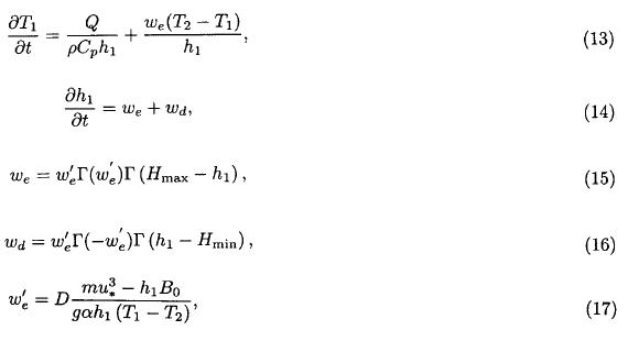
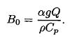
where hi is the upper layer thickness, u* is the friction velocity, m is the wind stirring coefficient, B0 is the buoyancy flux, g is gravity acceleration,  is the coefficient of thermal expansion, T1 and T2 (constant in this case) are the temperatures of the upper and intermediate layer respectively. The entrainment is we and the detrainment wd. D is a coefficient that controls the rate of entrainment and detrainment, Hmax and Hmin restricts h1 to a predefined thickness range. Γ(x) is a Heaveside step function, where Γ(x) = 1 when X > 0, otherwise Γ(x) = 0. The buoyancy flux is a function of the surface heat flux and was computed as
Entrainment and detrainment change h1 toward the Monin-Obukhov thickness, given by
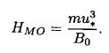
The Monin-Obukhov thickness corresponds to equilibrium between the terms in the numerator of the right hand side of equation (17). When B0 is positive and small, HMO is large. If B0≤ 0 then HMO = ∞ or negative and correspond to a water column that is mixed from surface to bottom. The Monin-Obukhov thickness is never reached because of the changing conditions. The rate at which h1 follows this thickness is controlled by the density difference relative to the intermediate layer, the wind stirring (mu*3), and the buoyancy flux (B0). It is also adjusted by the parameter D; for larger values of D the seasonal variability of h1 and T1 increase. This because as D increases entrainment enhances in winter and detrainment in summer producing thicknesses closer to their prescribed limits (i.e. Hmax in winter and Hmin in summer). Then, given the same seasonal heating the temperature variation is amplified as D is increased. On the other hand, the value of m heavily influences the average depth; for larger values the mean depth increases and the seasonal signal of temperature decreases due to the larger layer thickness.
Figure 2 shows the seasonal variation of the mixed layer thickness and temperature computed with the model defined by equations (13) to (17). Results illustrate the variation of the seasonal range of the mixed layer thickness and temperature for two different values of the parameter D. For this example we use the average surface heat fluxes and winds in the gulf from Tables 2, 3, 4, and 5, other values are those on Table 1.
2.2.2. The model mixed layer
To compute the entrainment (we) and detrainment (wd) in the numerical model we use the following expressions:
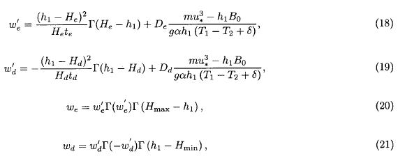
where He and Hd are limiting depths for entrainment and detrainment respectively, te and td are the relaxing time for entrainment and detrainment, De and Dd are coefficients that control the rate of entrainment and detrainment respectively, δ is a constant to prevent overturning, and all other variables have been previously defined.
The first term in the right hand side of equation (18) becomes important in upwelling regions and eliminates numerical singularities avoiding zero thickness of layers. This term has been used by several authors (for example McCreary and Kundu, 1988). The second term in the right hand side of (18) is a Niller and Kraus (1977) term. It involves h1, the surface buoyancy flux, the density difference between upper and intermediate layers, and wind stress; it is weaker than the first term, but is active during seasonal periods in wide areas, making its contribution important in the seasonal scale.
Equations (20) and (21), through the values of Hmax and Hmin, restrict entrainment and detrainment to a priori determined range of the mixed layer. They also prevent numerical instabilities produced from a very thin or thick mixed layer due to extreme conditions in buoyancy or turbulent kinetic energy production.
2.3. Numerical experiments
Several numerical experiments have been accomplished with the purpose of recognizing the relative contribution on the temperature variability of the advection and the entrainment. In all the experiments the model is forced with the wind stress and the Yucatan Current producing an eddy shedding period of 8.5 months. In each experiment we spin-up the model for one model year from an initial state of rest to reach stable conditions, then we use the following 12 years to extract the mean annual cycle. Experiment E-0 was carried out to quantify the contribution of the entrainment-detrainment to the seasonal variability of the SST. In this experiment all the terms in both, the heat equation and entrainment-detrainment equations are included. Experiments E-1A and E-1B show the contribution to the SST of the radiative fluxes estimated by bulk formulae and satellite respectively. In Experiments E-1A and E-1B all the terms in the heat equation and only the first term in the right hand side of equations (18) and (19) are included. Experiment E-2 was accomplish in order to quantify the contribution of the heat advection to the SST. In this experiment the advection terms in the temperature equations (5) and (9) are removed and only the first term on the right hand side of equations (18) and (19) are considered.
3. Heat fluxes
The heat fluxes through the surface are computed by the equation

where Q is the total heat flux through the surface. The first two terms in the right hand side of equation (22) are usually called radiative fluxes and the last two the turbulent heat fluxes.
The radiation fluxes (Qs + Qb) were estimated from the satellite data of Darnell et al. (1992), and in an independent way, following the equations proposed by Reed (1977, 1983). The selection of these formulae is supported by the review of Katsaros (1990). The computation of the turbulent fluxes was done using the equations given by Gill (1982) choosing constant turbulent coefficients consistent with the results of Geernaert (1990) (CE = CH = 1.4 x 10⁻³). A description of the formulae used is in Appendix I.
3.1. Discussion on heat flux estimates
Heat fluxes were computed for each point in a 2° x 2° grid and, from them, the mean surface heat flux per unit area for the entire gulf. The mean heat flux values obtained with these formulae are shown on Figure 3 together with previous results from H68, E83, and A93. Our results have a similar seasonal variation than those of previous works but with higher values during all the year. Moreover, differences are larger in winter compared to E83 or A93, and in summer when are compared to H68 (Fig. 3, Table 2).
These differences are smaller than the seasonal signal but they are significant compared to the expected interannual variability. They also have consequences on the role that the gulf has in the northward heat transport. We review the estimation of each term in the heat equation. Unfortunately not all previous works separate the short-wave and long-wave radiation nor the latent and sensible heat fluxes considering them together as radiative and turbulent fluxes respectively.
3.1.1. Radiative fluxes
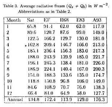
The radiative flux estimates are represented on Figure 4 and Table 3. There are three previous estimates (E83, H68, and A93) and the two computed here: one using Reed's formulae with data from COADS as input, and another using radiation measured by satellite (Darnell et al., 1992). The data produced by Reed's formulae have the largest mean value, and are larger during all the year than the values proposed by E83 and H68. Differences increase in summer reaching more than 100 W m-2 between H68 and those obtained following Reed's formulae.
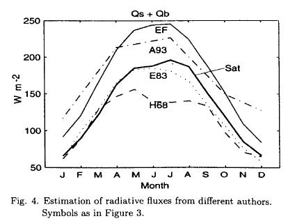
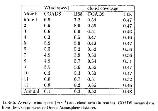
The short-wave radiation in cloudy sky has been computed with many formulae giving significant differences. The computation of the cloud attenuation to the short-wave radiation is one of the main causes of disparities, it has been computed as a linear or nonlinear function of cloudiness with different coefficients (Katsaros, 1990). Another difference between the short-wave radiation estimates is due to the fact that some formulae also include the angle of declination of the sun in the computations. We choose Reed's formulae since Katsaros (1990) underlines that this formula better agrees with direct measurements. The values obtained with this formula are considerably higher than those obtained following the formula from Budyko (1974), which is the same used by Etter (1983). The term related to the sun declination in Reed's formula induces larger differences in the summer. As an example, if Budyko's and Reed's formulae are used with the same Qc (clear sky radiation) and cloudiness at 25° N, there is a mean annual difference of 33 W m-2 (Fig. 5). On the other hand, using Reed's formula, a difference of 13% in cloud cover (from 52% obtained using COADS data to 65% used by A93) induces a difference of 23 W m-2 on the annual mean (Fig. 5).
The long-wave radiation estimation formulae differ because the black body radiation is multiplied by an absorption function which depends on the cloud cover and the humidity. The absorption function has different parameterizations in the formulae of each author.
The surface heat fluxes obtained using satellite radiation data are similar to those reported by E83, larger for summer than those of H68 and lower all the year than A93 (Table 3). These data were computed from a two year data set (1987-1988). Using these data to compute the total surface heat fluxes, the monthly values are also similar to E83 and slightly larger than A93 and H68 (Fig. 3). The net mean surface heat flux is 9.0 W m-2.
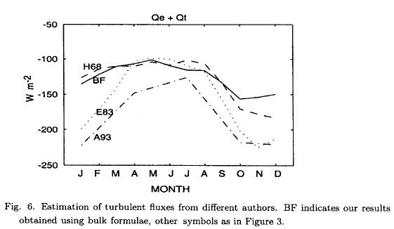
3.1.2. Turbulent fluxes
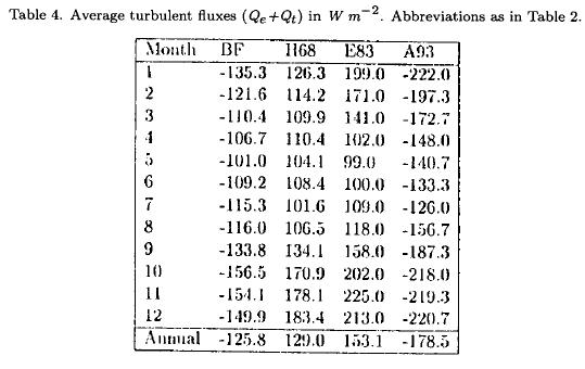
The formulae that we used in the computation of the turbulent fluxes are similar to those used in previous studies in the Gulf of Mexico (H68; E83; Etter et al, 1987; A93) but with different turbulent coefficients. These authors had used very different values (Appendix III), which produce significant differences. The estimation of the turbulent fluxes is linear in the turbulent coefficient. In the Gulf of Mexico an increment in CE and CH of 0.1 x 10⁻³ in the turbulent coefficients of the latent and sensible heat flux equations produces a decrease in the annual mean flux of ~10 W m-2. Recent experiments (Geernaert, 1990) show that the best approximations are linear functions of the wind speed. We use a constant value for the turbulent coefficients of CE = CH = 1.4 x 10⁻³ corresponding to tropical areas for wind speed of 10 ms-1.
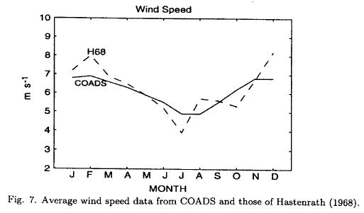
Figure 6 shows our estimates of monthly means of the turbulent fluxes together with those of previous works. Our values are lower than those obtained by A93 and E83. The seasonal signal is more intense in the E83 and A93 calculations. The higher seasonal variation on the E83 turbulent fluxes could be due to the fact that he used variable coefficients which increase the turbulent fluxes in winter, when the wind speed is stronger. A93 used a constant coefficient CE and CH = 1.6 x 10⁻³, a value between the one used by H68 and E83, but they obtained the strongest turbulent fluxes (Table 4 and Fig. 6). The large values estimated by A93 might be due to the wind data that they used (from the US Weather Bureau, 1952). Unfortunately they do not include in their paper the values of the wind data itself. The wind speed data used by H68 are similar to COADS, as can be seen on Figure 7. However, in both cases, it has to be considered that both data sets could underestimate the turbulent fluxes since they are from ships, and ships tend to avoid storms.
4. Modeling the sea surface temperature
The SST was analyzed with the numerical model described in section 2. The heat fluxes into the model are prescribed using equation (12). To study the seasonal behavior we suppressed the variability due to propagating eddies by taking the monthly mean temperature over 12 years of monthly model data.
4.1. Radiation estimated from satellite and empirical formulae
Experiments E-1A and E-1B have the same mixed layer physics, but different heat input sources. In experiment E-1A the radiation fluxes were computed with the empirical formulae of Reed (1977, 1983). In the output of this experiment the average temperature stays higher than the observed during all year with a difference in the mean temperature of 1.9°C and a root mean square (RMS) error, relative to observations, of more than 2.5°C.
In experiment E-1B the radiation fluxes estimated from satellite were used in the computation of the surface heat fluxes. In this case the average model temperature has a mean difference to the average temperature of observations of 0.6°C, with a RMS error relative to observations of 1.47°C.
As we have shown, there are considerable differences in the estimation of the radiation fluxes using Reed's formulae and those from satellite. If the computations using Reed's formulae were correct, with a transport of 25 Sv and considering as a good approximation that all the heat gained is exported through the Strait of Florida, there must be an average difference of 0.5°C between the temperatures of inflowing (at the Yucatan Channel) and the outflowing (through the Strait of Florida) water temperatures. If we consider that the temperature changes are limited to the upper 300 m and the transport in this layer is of 12 Sv (Gallegos et al, 1998), the temperature difference must be 1°C.
The studies that refer to the heat transport in the Yucatan Channel and Strait of Florida do not indicate those temperature differences (H68). On the other hand, in E-1A, which was ran with the data from Reed's formula, the model temperature remained higher than observations indicating that the heat advection through the Strait of Florida, necessary to decrease the Gulf temperature, is not there.
Based on these results we decide to perform our experiments using the satellite radiation data as the best approach.
The SST in E-1B is determined mainly by air-sea interaction and heat advection. In this experiment, vertical fluxes between the upper and the intermediate layers are limited to small regions where there are strong boundary currents.
E-1B reproduces qualitatively well the most important characteristics of the SST in the Gulf of Mexico. Model SST data are higher than COADS data from October to March and lower from April to September.
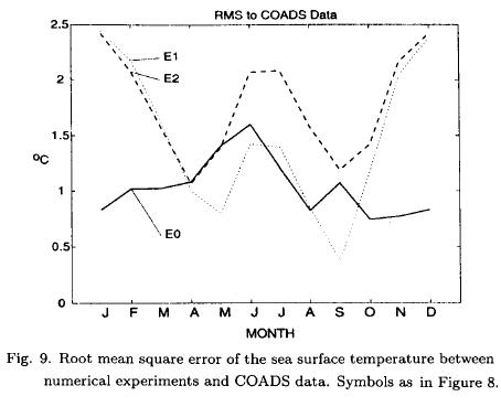
The mean temperature of model results is similar to the mean temperature of observations, with differences between them with an average of 1.3°C (Fig. 8) and a RMS of 1.47°C (Fig. 9). In winter, model temperatures are higher than COADS-SST, and differences reach more than 2.5°C in the northern gulf. The maximum model temperature is reached in September, lagging one month the maximum of COADS data; the minimum occurs in February as in observations. The lag in the SST cycle can be explained by the fact that in the model the surface heat is distributed instantaneously over the entire upper layer instead of progressively, diffusing it from the surface, in which case the SST responds faster.
4.2. Advection and entrainment-detrainment contributions to the SST change
In E-2 the advection terms on the heat equation are removed and the SST is determined solely by air-sea interaction. The mean spatial temperature is similar to that of E-1B. The Loop Current and eddies temperature signal disappears, while north-south temperature gradients are more intense. In winter and spring the temperature at the northern gulf are lower than in E-1B, and remain closer to observations, but in other regions temperatures are higher and consequently produce a similar RMS (Figs. 8, 9).
The higher winter temperature of the model, both E-1B and E-2, compared to observations, suggests that there are other important cooling processes besides the interaction through the sea surface and advection.
In E-0, we included an entrainment-detrainment process associated to surface fluxes that simulate the seasonal thickness change of the mixed layer. The seasonal variation of the SST is better reproduced when entrainment is included because it contributes to the winter cooling. The RMS from E-0 upper layer mean temperature to observations has an average of 1.0°C while E-1B and E-2 have 1.5°C and 1.7°C, respectively (Figs. 8, 9).
Our results differ from A93 in that they consider a mixed layer of constant depth (60 m) and vertical fluxes negligible below this depth. The main difference is due to the turbulent fluxes that they have, which are considerably stronger than ours. They use a larger turbulent coefficients (CE = CH = 1.6 x 10⁻³) than the ones that recent experiments suggest, and a different wind speed data source.
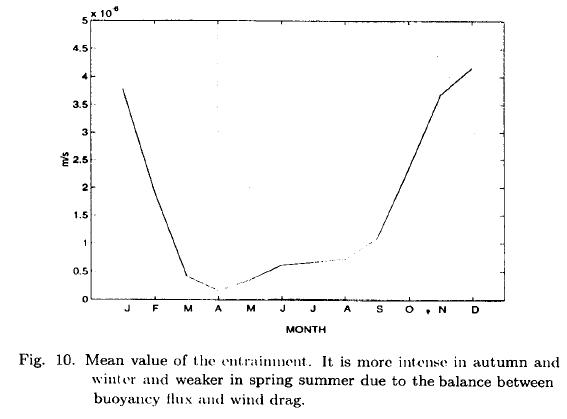
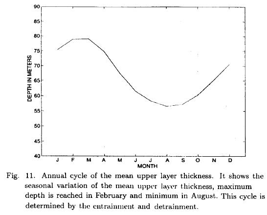
The annual cycle of the mean value of the entrainment is represented in Figure 10. Entrainment is stronger during October and November. The mean thickness of the mixed layer is represented in Figure 11 showing that deepening of the upper layer begins in late September and ends in February, reaching its maximum rate of change in November. Another evidence of entrainment is reviewed in section 4.4.
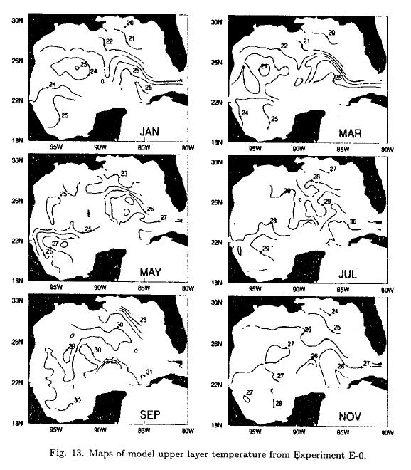
4.3. Seasonal sea surface temperature variability
Monthly SST from COADS and model upper-layer temperature from E-0 show lower values in February and maximum in August-September (Figs. 12 and 13). The SST begins to rise in March at the same time that the mixed layer thickness begins to decrease and the heat flux through the surface becomes positive (Figs. 3, 8, 12, 13). In March, after the previous winter season, there are strong north-south gradients. The anticyclonic eddies and the Loop Current are clearly identifiable in SST (removed on figures 12 and 13 since they are monthly composite means), due to the higher temperature than their surrounding. Meanwhile, the Bay of Campeche has higher temperatures than the northern gulf. However, in the middle of the Bay of Campeche the water is cooler than its surroundings due to a cyclonic circulation. In the Bay of Campeche, the model temperatures are higher than observations. A review of the causes shows that, during winter, the COADS winds are low and cloud cover fields show clear skies in the south and southeastern Bay of Campeche (there are few data values in the region) producing low heat loss by latent heat flux and strong heat input by short-wave radiation.
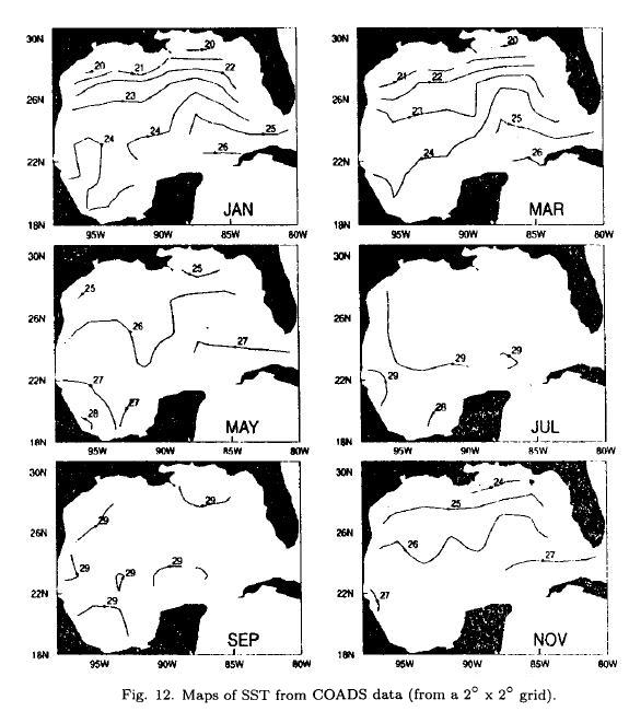
In May the downward heat flux is positive in the entire gulf, the SST still has some north-south gradients and the Bay of Campeche SST reaches 28°C. The Loop Current, their eddies, and the Strait of Florida gradient are still evident in SST.
In July the entire gulf has almost the same SST, between 28°C and 29.5°C making indistinguishable the Loop Current and the eddies through surface temperature observations due to the lack of temperature contrasts.
The scenario described for July continues until September, increasing the SST to 29°C or 30°C in the entire gulf. In October, the gulf starts to cool because the heat flux through the surface changes its direction. The winds are stronger and change to a more southwestward direction. In November, the heat loss to the atmosphere is more intense and in combination with stronger winds that rise the levels of turbulent kinetic energy produces entrainment, deepening and cooling of the mixed layer. The cooling mechanisms are not spatially homogeneous; entrainment is more intense in the northern and western gulf. The surface cooling and the inflow of subsurface cold waters increase the SST gradients and the anticyclonic eddies and the Loop Current have higher surface temperature than their surroundings. Also, a cold signature in the western Bay of Campeche can be seen due to the cyclonic circulation in the region (Fig. 13). Entrainment in the upper layer continues until February, cooling and deepening the mixed layer, and increasing the SST gradients.
4.4. Evidence of entrainment
We look for an independent evidence of the existence of the entrainment in the concentration of pigment values from the satellite images processed by NASA's Goddard Space Flight Center (Tran et al, 1992). Pigments in the Gulf of Mexico are more intense in the shelf area and near the river mouths, with weaker values in the deep areas. Figure 14 presents the monthly average values for regions off the shelf. The pigment concentrations in the inner gulf are weak but show a clear seasonal signal with higher values in winter and spring and lower in summer in agreement with the results obtained for the entrainment. Pigment estimations from Tran et al. (1992) data are similar to those of Müller et al. (1991) and Walsh et al. (1986). The correspondence in phase of the pigment and the entrainment cycle does not prove that this mechanism is the cause of a fraction of the winter cooling but it reinforces the hypothesis.
The mechanism that we proposed implies that a fraction of the heat gained by the gulf through the surface is transferred by detrainment into intermediate waters and exported through the strait.
5. Discussion and final remarks
The heat fluxes in the Gulf of Mexico were reviewed using a 2½ numerical layer model with thermodynamics and mixed layer physics and through the analysis of bulk formulae, climatological data from COADS and radiation estimations from satellite. Heat fluxes estimate was compared with those of previous studies.
The numerical model was forced by a constant inflow and outflow through the Yucatan Channel and the Strait of Florida respectively, and monthly climatological winds. Monthly heat fluxes through the surface were parameterized as Haney (1971). Different versions of the entrainment parameterization and the heat equation were used to determine the influence of different physical processes on the SST. Also, the contribution of each term in the heat equation was reviewed by examining its impact on the modeled SST.
It is shown that the use of different formulae to compute the short wave radiation results in considerable uneven estimations. Results are very sensitive to changes in the cloud cover value and its parameterization. This analysis shows that the satellite radiative estimates are good for the radiative fluxes. The computation of the long wave radiation is sensible to the black body absorption function, which varies depending on cloud cover and humidity values. In addition, it is shown that turbulent fluxes are highly dependant on the values of the turbulent coefficients in the empirical formulae. Based on the review of different parameterizations of the turbulent fluxes discussed by Geernaert (1990), we choose values for the turbulent coefficients that are smaller than those considered in previous works.
In order to analyze the relative influence of different processes on the SST, several numerical experiments were conducted including or removing terms in the model equations. When temperature advection is removed (E-2), the SST shows significant changes, relative to the case in which it is included (E-1B), mostly in the northwestern gulf where the advection of water from the south increases winter temperatures. However, when entrainment-detrainment associated with the wind stress and the buoyancy flux are included (E-0), the winter temperatures are better reproduced and the RMS error between modeled and observed SST decreases to almost half of that in E-1B.
A mean net heat flux of 9.0 W m-2 is estimated, the composite year with the mean removed has a maximum value in May (84.1 W m-2), remaining almost with the same value until July and has a minimum in December (-83 W m-2). It is shown that differences between our estimate of the heat fluxes and those of previous studies are due to different data sources and algorithms used in the computation. Another possible source of differences with E83 is the lack of data in the Bay of Campeche in his work.
It is shown that the entrainment and detrainment (shallowing and deepening of the mixed layer) have a significant role in the seasonal evolution of the sea surface temperature of the Gulf of Mexico. In addition, the entrainment seasonal cycle, characterized by an increase in winter and a decrease in summer, agrees with the pigment cycle as is expected by the input of subsurface water rich in nutrients into the mixed layer.
Acknowledgements
Jorge Zavala received a scholarship from CONACyT. This work was supported by CONACYT grants 28799T and 28794T, and CICESE's normal funding. Comments by E. Pavía, F. Graef, P. Ripa and R. Castro helped substantially during this study. We thank J. Sheinbaum for his advice on numerical and physical issues. S. Morey and M. Bourassa (COAPS/FSU) made important suggestions for the improvement of this manuscript. This research was completed under the support of The Center for Ocean-Atmospheric Prediction Studies which receives its base funding from ONR's Secretary of Navy Grant to Dr. James J. O'Brien.
REFERENCES
Adem, J., V. M. Mendoza, E. E. Villanueva-Urrutia, and M. A. Monreal-Gómez, 1991. On the simulation of the sea surface temperature in the Gulf of Mexico using a thermodynamic model. Atmósfera, 4, 87-99. [ Links ]
Adem, J., E. E. Villanueva-Urrutia, and V. M. Mendoza, 1993. A new method for estimating the seasonal cycle of the heat balance, with application to the Gulf of Mexico. Geofís. Int., 32, 21-34. [ Links ]
Adem, J., E. E. Villanueva-Urrutia, and V. M. Mendoza, 1994. Preliminary experiments on the prediction of sea surface temperature anomalies in the Gulf of Mexico. Geofís. Int., 33, 511-521. [ Links ]
Bernhart, F., and H. Philipps, 1958. Die räumliche und zeitkiche Verteilung der Einstrhlung, der Ausstrahlung und der Strahlungsilanz im Meeresniveau. Teil I. Abdandl. Meteorol. Hydrol. Dienstes DDR, 45, 257 p. [ Links ]
Budyko, M. I., 1963. Atlas of the Heat Balance of Earth. Academy of Sciences, Moscow, 69 pp. [ Links ]
Budyko, M. I., 1974. Climate and Life, International Geophysics Series, Vol. 18, Academic Press, 508 p. [ Links ]
Bunker, A. F., 1976. Computations of Surface Energy Flux and Annual Air-Sea interaction cycles of the North Atlantic Ocean. Mon. Wea. Rev., 104, 1122-1140. [ Links ]
Darnell, W. L., W. F. Staylor, S. K. Grupta, N. A. Ritchey, and A. C. Wilber, 1992. Seasonal variation of surface radiation budget derived from ISCCP-C1 data. J. Geophys. Res., 97, 15741-15760. [ Links ]
Dietrich, D. E., and C. A. Lin., 1994. Numerical studies of eddy shedding in the Gulf of Mexico. J. Geophys. Res., 99, C4, 7599-7615. [ Links ]
Dronkers, J., 1969. Tidal computations in rivers, costal areas and seas. J. of Hydraulics Division ASCE, 95, 44-77. [ Links ]
Elliot, B. A., 1982. Anticyclonic rings in the Gulf of Mexico. J. Phys. Oceanogr., 12, 1292-1309. [ Links ]
Emery, W. J., 1976. The role of vertical motion in the heat budget of the upper Northeastern Pacific Ocean. J. Phys. Oceanogr., 6, 299-305. [ Links ]
Etter, P. C., 1983. Heat and fresh water Budgets in the Gulf of Mexico. J. Phys. Oceanogr. 13, 2058-2069. [ Links ]
Etter, P. C., P. J. Lamb, and D. H. Portis, 1987. Heat and fresh water Budgets in the Caribbean Sea with Revised Estimates for the Central American Seas. J. Phys. Oceanogr., 17, 1232-1248. [ Links ]
Gallegos, A., I. Victoria, J. Zavala, M. Fernández, and I. Peiné, 1998. Hidrología de los Estrechos del Mar Caribe Rev. Invest. Mar., 19. [ Links ]
Geernaert, G. L., 1990. Bulk parameterizations for the wind stress and heat fluxes, on Surface waves and fluxes. Vol. I Current Theory, Chapter 4, edited by Geernaert, G. L., and W. J. Plant, Kluwer Academic Publishers. [ Links ]
Gill, A. E., 1982. Atmosphere-Ocean Dynamics, International Geophysics Series, Vol. 30. [ Links ]
Haney, R. L., 1971, Surface thermal boundary condition for ocean circulation models. J. Phys. Oceanogr., 1, 241-248. [ Links ]
Hastenrath, S. L., 1968. Estimates of the latent and sensible heat flux for the Caribbean and the Gulf of Mexico. Limnol. Oceanogr., 13, 322-331. [ Links ]
Hastenrath, S. L., and P. Lamb, 1978. Heat Budget Atlas of the Tropical Atlantic and Eastern Pacific Oceans. University of Wisconsin Press. 104. [ Links ]
Hellerman, S., and M. Rosenstein, 1983. Normal monthly wind stress over the world ocean with error estimates. J. Phys. Oceanogr., 13, 1093-1104. [ Links ]
Holland, W. R., 1978. The role of mesoscale eddies in the general circulation of the ocean-numerical experiments using a wind driven quasi-geostrophic model, J. Phys. Oceanogr., 8, 1093-1104. [ Links ]
Hurlburt, H. E., and J. D. Thompson, 1980. A numerical study of Loop Current intrusions and eddy shedding. J. Phys. Oceanogr., 10, 1611-1651. [ Links ]
Katsaros, K. B., 1990. Parameterization schemes and models for estimating the surface radiation budget, on Surface waves and fluxes. Vol. II Remote Sensing, Chapter 18 edited by Geernaert, G. L. and W. J. Plant, Kluwer Academic Publishers. [ Links ]
Kuhn, P. M., 1962. Radiometersonde measurements of water vapor flux emissivity. Ph.D. thesis, University of Wisconsin, Madison, 53 p. [ Links ]
Lavoie, R., 1972. A mesoscale numerical model of lake-effect storms. J. Atmos. Sci., 29, 1025-1040. [ Links ]
Levitus, S., 1982. Climatological Atlas of the World Ocean. NOAA Prof. Pap. [ Links ]
McCreary, J. P., Jr., and P. Kundu, 1988. A numerical investigation of the Somali Current during the Southwest Monsoon. J. Mar. Res., 46, 25-58. [ Links ]
McCreary, J. P., Jr., P. Kundu, and R. L. Molinari, 1993. A numerical investigation of dynamics, thermodynamics and mixed-layer processes in the Indian Ocean, Prog. Oceanog., 31, 181-224. [ Links ]
McCreary, J. P., Jr., and P. Lu, 1994. Interaction between the Subtropical and Equatorial Ocean Circulations: The Subtropical Cell. J. Phys. Oceanogr., 229, 466-497. [ Links ]
Mesinger, F., and A. Arakawa, 1976. Numerical methods used in atmospheric models. GARP Publications, 17. [ Links ]
Müller-Karger, F. E., J. Walsh, R. H. Evans, and M. B. Meyers, 1991. On the seasonal phytoplankton concentration and sea surface temperature cycles of the Gulf of Mexico as determined by satellites. J. Geophys. Res., 96, 12645-12665. [ Links ]
Niiler, P. P., and E. B. Kraus, 1977. One dimensional model of the upper ocean, in Modelling and prediction of the upper layer of the ocean, E. B. Kraus, Ed., Pergamon, 143-172. [ Links ]
Reed, R. K., 1977. On Estimating Insolation Over the Ocean, J. Phys. Oceanogr., 7, 482-485. [ Links ]
Reed, R. K., 1983. Heat fluxes over the eastern tropical Pacific and aspects of the 1972 El Niño, J. Geophys. Res., 88, 9627-9638. [ Links ]
Tran, A. V., E. Smith, J. Hyon, R. Evans, O. Brown, and G. Feldman, 1992. Satellite-derived multichannel sea surface temperature and phytoplancton pigment concentration data: a CD-ROM set containing monthly mean distribution for the global oceans, NOAA. [ Links ]
Seckel, G. R., and F. H. Beaudry, 1973. The radiation from sun and sky over the North Pacific Ocean (abstract), Eos Trans. AGU, 54, 1114. [ Links ]
Schopf, P. S., and M. A. Cane, 1983. On equatorial dynamics, mixed layer physics and sea surface temperature. J. Phys. Oceanogr., 13, 917-935. [ Links ]
Sturges, W., J. C. Evans, S. Wesch, S., and W. Holland., 1993. Separation of warm-core rings in the Gulf of Mexico. J. Phys. Oceanogr., 23, 250-268. [ Links ]
Vázquez, A. M., 1993. Bay of Campeche Cyclone, Ph D Thesis. Texas A & M University. [ Links ]
Vukovich, F. M., 1995. An updated evaluation of the Loop Current's eddy-shedding frequency. J. Geophys. Res., 100, C5, 8655-8659. [ Links ]
Vukovich, F. M., and B. W. Crissman, 1986. Aspects of warm rings in the Gulf of Mexico, J. Geophys. Res., 91, 2645-2660. [ Links ]
Walsh, J. J., A. D. Dieterle, M. B. Meyers, and F. E. Müller-Karger, 1989. Nitrogen exchange at the continental margin: A numerical study of the Gulf of Mexico. Prog. Oceanog. 23, pp 245-301. [ Links ]
Zavala, J. Ochoa, A. Parés-Sierra, and J. Sheinbaum, 1997. A Numerical study of the circulation and the sea surface temperature in the Gulf of Mexico. In Numerical simulations in the environmental and Earth Sciences, Ed. Fernando García et al., Cambridge. [ Links ]
Zavala, J. Ochoa, and A. Parés-Sierra, 2001. Seasonal circulation in the Gulf of Mexico: A numerical study. (Manuscript in preparation. [ Links ])

