An improved parameterization of the mean monthly precipitation in the Northern Hemisphere

 

V. M. Mendoza, B. Oda and J. Adem*

Centro de Ciencias de la Atmósfera, Circuito exterior, Ciudad Universitaria, C. P. 04510, México, D. F., México.
* Member of El Colegio Nacional

 

(Manuscript received May 31, 2000; accepted in final form Sept. 11, 2000)

 

RESUMEN

Se presenta una parametrización de la precipitación media mensual desarrollada en una ecuación de regresión linear múltiple en función de la temperatura y del viento horizontal. En el cálculo de los coeficientes de la ecuación se usaron los datos de un período de once años, de enero de 1982 a diciembre de 1992, de las anomalías medias mensuales de la precipitación, la temperatura, las componentes zonal y meridional del viento, y la verticidad. De esta ecuación se obtiene una habilidad de más de 80% en la estimación de las anomalías medias mensuales de la precipitación en el Hemisferio Norte. El presente método puede ser usado para pronosticar las anomalías mensuales de la precipitación con el modelo termodinámico de Adem, u otros modelos de balance de energía o de circulación general de la atmósfera, así como para calcular anomalías mensuales de precipitación a partir de datos de anomalías de temperatura y viento observados.

 

ABSTRACT

A mean monthly precipitation parameterization is given. It is developed by a multiple linear regression equation in terms of the temperature and the horizontal wind.

Using a period of eleven years, from January 1982 to December 1992, for the anomalies of the mean monthly precipitation, temperature, zonal and meridional wind, and vorticity of the wind as variable data, we have obtained a skill above 80% in the estimation of the mean monthly precipitation anomalies in the Northern Hemisphere.

The parameterization may be used to predict monthly precipitation anomalies with the Adem's Thermodynamic Model, or with any others energy balance or general circulation models, as well as to compute monthly precipitation anomalies from observed anomalies of temperature and horizontal wind data.

 

1. Introduction

In the early sixties Adem (1964, 1965) developed a time averaged thermodynamic model for monthly and seasonal prediction. Since that time the Adem's model has been succesfully used to simulate the temperature and precipitation anomalies of past and future climates and to estimate the effect of the increase of the atmospheric CO₂ on the climate; as well as to make monthly and seasonal predictions (Adem, 1970; Adem, 1991; Adem et al, 1995; Adem and Garduño, 1998; Adem et al, 2000). In support for this model Clapp et al. (1965), derived a parameterization of the monthly anomalies of precipitation in the Northern Hemisphere as a function of the temperature anomalies and horizontal components of the wind at the 700mb level.

He used a multiple regression procedure to compute the coefficients which were functions of the season and the geographical coordinates.

Furthermore, where data were not available, he used the empirical climatological knowledge, according to the region and the local climate.

Previous studies by Smith (1942), Stidd (1954), and Klein (1963) showed that rainfall could be especified from the mean circulation parameters chosen in the parameterization.

The results of using the parameterization of Clapp et al. (1965) to simulate and predict the precipitation anomalies have been very encouraging. Since that time, several studies about models of rainfall, gauge observations, and the difficulties of the indirect estimation of the precipitation have been published (Drufuca and Zawadzki, 1975; Smith and Karr, 1985; Arkin and Meisner, 1987; Xie and Arkin, 1996). A theoretical study was carried out by Mendoza et al. (1998), obtaining a linear parameterization of the precipitation anomalies as a function of the surface temperature, the 700mb temperature anomalies and the 700mb horizontal wind anomalies. Four correlation mean monthly variables were found as the most significant: the temperature, the 700mb horizontal, zonal and meridional wind components, and the corresponding vorticity.

Therefore, in the present work we have used a linear multiple correlation procedure, similar to that suggested by Clapp et al. (1965), with the best available data, to derive parameterizations with all or some of these variables, in order to determine which combination of them yields the best results. Furthermore, instead of the horizontal wind component terms we also try the derivatives of 700mb temperature with respect to the x and y horizontal coordinates, which are used in the energy balance models where the wind is computed from the temperature field (Adem, 1967).

 

2. The statistical parameterization

The well known matrix theory and least squares method to correlate the data, (Courant and John, 1984; Spiegel, 1961), were used to construct a linear multiple regression equation, which expresses the monthly precipitation anomalies in terms of the monthly anomalies of the temperature, the zonal and meridional wind, and the vorticity at 700mb level.

The linear multiple regression equation can be expressed as:

where α,b,c,d, and e, are the correlation coefficients, P is the mean monthly precipitation anomaly; T is the mean monthly temperature anomaly at the 700mb level; u and v are the anomalies of the mean monthly zonal and meridional components of the wind at the 700mb level, and is the corresponding vorticity anomaly. The positive x and y directions are from West to East and from South to North, respectively. These variables have been chosen because they were found to be the most significant variables according to the theoretical precipitation parameterization analysis (Mendoza et al, 1998).

The independent term a is the residual precipitation term due to atmospheric or surface variables not considered in the development. This term results to be negligibly small as the numerical experiments will show below.

For the models in which the wind is computed from the temperature field, we have derived an equation, similar to the equation of Clapp et al. (1965), in which the wind components at 700mb can be replaced by temperature gradients at the same level. The equation is expressed by:

where, u_T , v_T and are the anomalies of the zonal and meridional wind and the vorticity of the wind, respectively.

The components of the wind anomalies are given by:

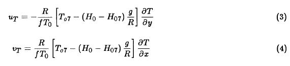
where R is the perfect gas constant; T₀ = 229.5K; T₀₇ = T + Γ (H₀ - H₀₇); H₀ = 9km, and H₀₇ = 3km, Γ is the lapse rate in middle latitudes, f is the Coriolis parameter, and g is the gravitational acceleration. In the derivation of equations (3) and (4) we are using the geostrophic wind approach, hydrostatic equilibrium, perfect gas, constant lapse rate and the assumption of constant density at the top of the atmospheric layer of depth H₀ (Adem, 1967, 1970).

 

3. Numerical experiments

For the determination of the linear regression coefficients of Eqs. (1) and (2), we used the NCEP/NCAR Reanalysis CD Rom data for the mean monthly anomalies of precipitation, temperature and winds at the 700mb level, during the months from January 1982 to December 1992 (eleven year period). We computed the regression coefficients of both equations, for each month and each one of 1977 points of the grid, in the NMC polar stereographic proyection of the Northern Hemisphere.

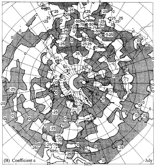
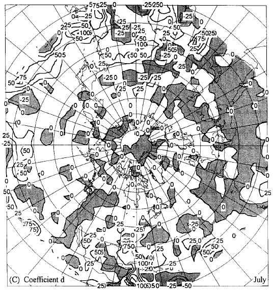
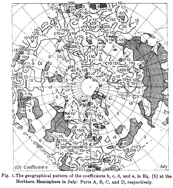
To illustrate the role of each term in the parameterization of the precipitation we have used the summer period. The geographical patterns of the coefficients b, c, d and e for this season are shown in Figure 1 in parts A, B, C and D, respectively. From this figure we can make some observations similar to those made by Clapp et al. (1965). The geographical pattern of the temperature coefficient b, depends mainly on climate anomalies. Over continents and oceans for all seasons, precipitation tends to occur with above normal temperature where b is positive; and with below normal temperature, where b is negative. Therefore, as shown in Figure 1 A, in summer and at lower latitudes, precipitation tends to occur with above normal temperature over Mexico and Central America, over the Indie Ocean and the west parts of the Pacific Ocean.

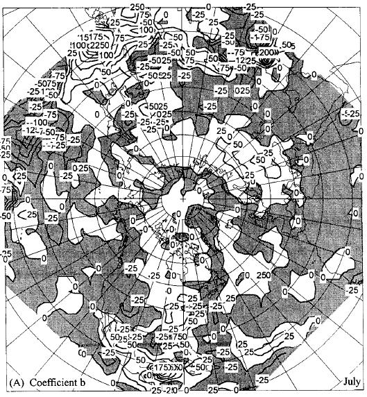
The same is truth in the middle latitudes where the precipitation tends to occur with above normal temperatures in the east coasts of U. S., Canada, Europe, mediterranean area, and Asia. Otherwise over the west coasts of those regions, the precipitation tends to occur with below normal temperature. Over desertic regions, precipitation tends to occur with below normal temperature at all seasons. These associations are due partly to the influence of cloudiness on long and short-wave radiation.

The distribution of the coefficients of the wind components depends mainly on the terrain and latitude. Where westerly or southerly wind is directed from water to land and especially if it is forced to ascend mountains, there is a strong positive relationship between rainfall and wind speed at the west coast of both continents except over Africa. When directed downslope, these components are negatively related to rainfall. Over southern oceans, for all seasons, heavy rain occurs with easterly winds in conformity with observed rainfall in easterly waves and tropical storms, and with the distribution of the coefficient c in lower latitudes (Fig. 1B).

The south-north wind component tends to be positively related to rainfall almost everywhere due to the observed fact that convergence and rising motion prevails with southerly winds and the opposite with northerly winds. From the summer map (Fig. 1 C) of coefficient d, it is assumed that the regions of the North-African continent and part of U. S. and Europe, where d values are negative, the rainfall tends to occur with negative anomalies of meridional wind.

From the coefficient e map, which is shown in Figure 1 D for summer, we can see that the values are positive in almost the whole Northern Hemisphere. The figure shows the whole Eurasian continent positively correlated with the above normal vorticity for the rainfall. Otherwise over the American continent, over the west part of U. S. and its Pacific coast, the precipitation tends to occur with negative anomaly of the vorticity. Over Africa, in the Northern Hemisphere, the coefficient e is negative for all seasons.

Next we will carry out experiments to evaluate the significance of the independent term a and of the vorticity term in Eq. (1). For this purpose we use two modified forms of Eq. (1): the equation

where the independent term a is neglected, and equation

where both eζ and a are neglected.

Furthermore, we modify Eq. (2) neglecting the α' term, obtaining

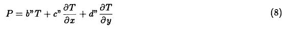
Finally, we will also test the the formula of Clapp et al. (1965)

We have carried out several experiments to evaluate the skill of the parameterizations (1), (5), (6), (7) and (8). The measure of the skill is based on the so-called S₁ score (Teweles and Wobus, 1954), which characterizes the normalized error. We consider that an average score 0 is near perfect, while 50 shows little or no skill. The average skill in percentage is given by 2 X (50 — S₁), which yields 0 for a worthless chart and 100 for a virtually perfect one. In all of these experiments, the same period of eleven years data, from January 1982 to December 1992, was used.

The skill of the parameterization and the percentage of correctly computed signs of the precipitation anomalies using (5), are shown in Table 1 as EX0.

We evaluated the significance of the a term, comparing the average seasonal and annual skill using Eq. (1) with those using (5). The difference between the skill of these equations (EX1 in Table 1), is the significance of the a term. We obtain an average annual difference of 0.4% in the skill of the computed anomaly of the total precipitation in the Northern Hemisphere. The difference in the average annual percentage of signs correctly computed is 0.9%. From these results we concluded that it is negligibly small.

We compared the skill of Eq. (5) with that of (6). Their difference, shown in Table 1, EX2 column, is due to the lack of the vorticity term in Eq. (6). The difference in the average annual skill is 2.8% and the difference in the average annual percentage of signs correctly computed is 4.2%. Therefore, we conclude that the vorticity term is important.

We also have evaluated the validity of using Eq. (7), computing the difference in the skills of Eqs. (5) and (7), shown in Table 1, in the EX3 column. The difference in the average annual skill is 2.5% and the annual difference in the percentage of signs correctly computed is 2.9%.

In order to find out the regions in the Northern Hemisphere where this procedure could be used successfully, we carried out another experiment. It consists in evaluating the skill of Eq. (5) in continental and oceanic regions separately, and using also the same data period. The results are shown in Tables 2 and 3, where we can see that regions like the American and the European continents and the Pacific and the Atlantic oceans evaluated with the S₁ score skill, yields an average seasonal and annual skill of around 75%; and around 80 and 90% for the Asian and North-African continents, respectively.

In another experiment, we have compared the skill of Eqs. (5) and (7) with the skill of Eq. (8). In this experiment, we computed the precipitation anomalies for the whole NMC Northern Hemisphere grid, using the January and July months of 1996, 1997 and 1998 data, which are six months outside of the period where the regression coefficients were computed. The data was obtained from the NOAA-CIRES Climate Diagnostic Center, through the Web site. We see from the average results of this experiment, shown in Table 4, that Eq. (7) yields the best skill (83.4%), and that there is no significant difference between the skill of Eqs. (5) and (8), while in the signs correctly computed, Eq. (5) is the best with about 60%.

Figures 2 and 3 show the precipitation anomalies computed with Eq. (5), in parts A, and observed in parts B for January and July of 1996 respectively. Table 4 shows that, in this case, for January the skill of the method is 81.6% and the percentage of signs correctly computed is 60.6%. For July, these values are 73.9 and 60.0%, respectively.

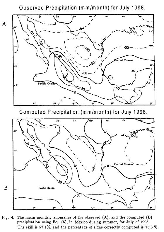
Our regional interest is Mexico, with its semi-tropical climate in the South, and semi-desertic in the North. Since the rainy season is the summer in Mexico, we computed as an example, the precipitation anomalies for July 1998, using Eq. (5) with the NOAA-CIRES CDC data. Figure 4 shows the mean monthly anomaly of the observed rainfall (part A), and the corresponding computed anomaly (part B), for July 1998 in Mexico. The corresponding skill for this case is 57.1%, and the corresponding percentage of the signs correctly computed is 73.3%.

 

4. Concluding remarks

From the annual skill of Eqs. (l), (5), (6) and (7) shown in Table 1, we obtain the following conclusions:

1. The difference in the annual average skill using Eq. (1) instead of (5) is 0.4%, and the corresponding difference in the annual average percentage of signs correctly computed is 0.9%. From these results it was concluded that the independent term a of Eq. (1) is negligibly small.

2. The difference in annual average skill using Eq. (5) instead of (6) is 2.8%, and the corresponding annual difference in percentage of signs correctly computed is 4.2%. These differences show the importance of the vorticity term in Eq. (5). Therefore, it was concluded that the use of Eq. (5) is better than that of both Eqs. (1) and (6), and that the four correlation variables in Eq. (5) are the best selection.

3. Using Eq. (5), we obtain 84.8% in the annual average skill, and 76.6% in the annual average percentage of signs correctly computed in the Northern Hemisphere. Therefore, it is a useful regression equation for the precipitation forecasting with models which predict the temperature, as well as the winds. Furthermore, Eq. (5) can also be used to estimate the precipitation anomalies from the temperature and horizontal wind data.

Furthermore, Tables 2 and 3 show that over the four continents as well as over the Pacific and the Atlantic oceans the evaluation yields a skill above 75%.

4. For the differences between using Eqs. (5) and (7), shown in Table 1, in EX3 column, we obtain 2.5% and 2.9% in the average annual percentage of skill, and the signs correctly computed, respectively, which compared with the corresponding skills obtained using Eq. (5), (84.8 and 76.6%), show that the option of Eq. (7), is good for some energy balanced models which predict only the temperature.

5. For January and July, of the years 1996, 1997 and 1998, the comparison of the results using Eq. (7) with those using Eq. (8) of Clapp et al. (1965), shows that the best skill is obtained with Eq. (7), with an appreciable skill difference of 8.3% between them (Table 4).

6. From the comparison of the results obtained from Eq. (5), with those of Eqs. (7) and (8) shown in Table 4, we conclude that for these illustrative 6 cases, the use of temperature gradients in the parameterization of the precipitation is as good as the use of the horizontal wind.

 

Acknowledgements

The data was obtained through the Web site by the NOAA-CIRES Climate Diagnostics Center, Boulder, Colorado ( http://www.cdc.noaa.gov/).

The authors thank Francisco J. Villicaña and E. E. Villanueva for some constructive comments that helped to improve this paper.

 

REFERENCES

Adem, J., 1964. On the Physical basis for the numerical prediction of monthly and seasonal temperature in the Troposphere-Ocean-Continent system. Mon. Wea. Rev., 92, 91-104.         [ Links ]

Adem, J., 1965. Experiments aiming at monthly and seasonal numerical weather prediction. Mon. Wea. Rev., 93, 495-503.         [ Links ]

Adem, J., 1967. Relations among wind, temperature, pressure and density, with particular reference to monthly averages. Mon. Wea. Rev., 95, 531-539.         [ Links ]

Adem, J., 1970. Incorporation of advection of heat by mean winds and by ocean currents in a thermodynamic model for long-range weather prediction. Mon. Wea. Rev., 98, 776-786.         [ Links ]

Adem, J., 1991. Review of the development and applications of the Adem thermodynamic model. Climate Dynamics, 5, 145-160.         [ Links ]

Adem, J., 1996. On the seasonal effect of orbital variations on the climates of the next 4000 years. Ann. Geophysicae, 14, 1198-1206.         [ Links ]

Adem, J., and R. Garduño, 1998. Feedback effects on the atmosphere CO_2– induced warming. Geofis. Int., 37, 55-70.         [ Links ]

Adem, J., A. Ruiz, V. M. Mendoza, R. Garduño, V. Barradas, 1995. Recent experiments on monthly weather prediction with the Adem Thermodynamic Model, with especial emphasis in Mexico. Atmosfera, 8, 23-34.         [ Links ]

Adem, J., V. M. Mendoza, A. Ruiz, E. E. Villanueva, R. Garduño, 2000. Recent numerical experiments on three-months extended and seasonal weather prediction with a thermodynamic model. Atmósfera, 13, 53-83.         [ Links ]

Arkin, P. A., B. N., Meisner, 1987. Spatial and annual variations in the diurnal cycle of large-scale tropical convective cloudiness and precipitation. Mon. Wea. Rev., 115, 2009-2031.         [ Links ]

Clapp, P. F., S. H. Scolnick, R. F. Taubensee, and F. J. Winninghoff, 1965. Parameterization of certain atmospheric heat sources and sinks for use in a numerical model for monthly and seasonal forecasting. Internal report, Extended Forecast Division (Available on request to Climate Analysis Center, NWS NOAA, Washington, D.C. 20233).         [ Links ]

Courant, R., F. John, 1984. Introducción al cálculo y al análisis matemático Vol. II, Ed. LIMUSA, S.A., Méx., 1041 pp.         [ Links ]

Drufuca, G., I. I., Zawadzki, 1975. Statistics of raingage data. Jour. App. Meteor., 14, 1419–1429.         [ Links ]

Klein, W. H., 1963. Specification of precipitation from the 700 milibar circulation. Mon. Wea. Rev., 91, 527-536.         [ Links ]

Mendoza, V. M., B. Oda, and J. Adem, 1998. Parametrization of the precipitation in the Northern Hemisphere and its verification in Mexico. Ann. Geophysicae, 16, 853-865.         [ Links ]

Smith, K. E., 1942. Five day precipitation pattern in the United States in relation to surface and upper-air mean charts. M.I.T. Cambridge, Mass., 144 pp. (Master's Thesis).         [ Links ]

Smith, J. A., A. F. Karr, 1985. Statistical inference for Point Process models of rainfall. Water Resour. Res., 21, 73-79.         [ Links ]

Spiegel, M. R., 1961. Statistcs, Schaum's outline series, Mc. Graw-Hill Book Co., N.Y., 359 pp.         [ Links ]

Stidd, C. K., 1954. The use of correlation fields in relating precipitation to circulation. Jour. Meteor., 11, 202-213.         [ Links ]

Teweles, S., H. Wobus, 1954. Verification of prognostic charts, Bull. Amer. Meteor. Soc., 35, 455-463.         [ Links ]

Xie, P., P. A. Arkin, 1996. Analyses of global monthly precipitation using gauge observations, satellite estimates, and numerical model predictions. Jour. Cli., 9, 840-858.         [ Links ]