


 nova página do texto(beta)
 Inglês (pdf)
 Artigo em XML
 Referências do artigo
 Enviar este artigo por email
 Citado por SciELO
  Similares em
SciELO
Similares em
SciELO 
 Permalink
INTRODUCTION
Climate change triggers severe negative effects on the global water resources (Fares et al., 2015). As the earth atmosphere warms, it is unclear how the precipitation will change or how these changes will impact regional rainfall (Ferreira et al., 2018). In fact, changes in rainfall distribution have attracted much attention because of the vulnerability of human activities to hydrological extreme events such as flood-producing rains and droughts (Kharin et al., 2007; Angheluţă and Badea, 2015). Recent record-breaking rainfall events in the last decade have occurred around the world causing severe impacts to human society and the environment including agricultural losses and flooding (Lehmann et al., 2015). Moreover, changes in water availability or more importantly the shortage of water in the future could have negative impacts on hydropower generation and on agricultural activities in Central America and México (Karmalkar et al., 2011). This is the case of arid and semiarid land areas (150 000 ha) of the Zacatecas state, located in Central México.
Zacatecas state is one of the most considerable providers of chili pepper and basic grains. It mainly provides dry beans and corn to the whole country. However, most of its cultivated land has a rain-fed agriculture and its aquifers are over-exploited with a deficit of about 201.1×10⁶ m3 per year (SEMARNAT, 2008). In this context, it is known that in countries where their economy is heavily dependent on low-productivity rain-fed agriculture, rainfall trends and variability are frequently mentioned factors in explaining various socioeconomic problems (Cheung et al., 2008). Thus, a better understanding of the spatial and temporal variability of rainfall, at local and regional scale, is paramount for advancing climate change research as well as for assessing the potential impacts of climate change on water resources (Nickl et al., 2010).
For the study of spatial and temporal variability of rainfall, several indexes have been developed. The Standardized Precipitation Index (SPI) has been used to categorize observed rainfall as a standardized departure with respect to a rainfall probability distribution function (McKee et al., 1993). This index has gained importance in recent years as a tool for climatic zone classification and a drought indicator. It allows performing comparisons across space and time (Naresh Kumar et al., 2009). The main advantage of this drought analysis technique is its simplicity and temporal flexibility. This index only uses records of the precipitation data over time (Mahfouz et al., 2016). Campos-Aranda (2015) used rainfall data registered at the weather station of Zacatecas, México and identified 39 droughts during 1953-2012 through the SPI; however, the author did not point out the involved SPI scale. In addition, Bautista-Capetillo et al. (2016) used rainfall data (period 2005-2014) from 111 weather stations located at the Mexico’s state of Zacatecas and identified different categories of drought by means of SPI’s at 3-, 6-, and 12-month scales; however, they considered that rainy season commonly start in April, however, that appears to be a dubious proposal. Nonetheless, SPI-based drought categories can be used to classify the Mexican territory in several zones as pointed out by Giddings et al. (2005). Therefore, it is possible to use the SPI to classify much smaller and more detailed zones. Hence, the aims of this study were: 1) To cluster monthly precipitation time series into groups that represent regions under the basis of similar precipitation regimes, 2) to compute regional Standardized Precipitation Indexes using all the members (time series) of each cluster, and 3) to estimate trends of the regional Standardized Precipitation Indexes.
MATERIALS AND METHODS
Precipitation Data
In this work, a database of long-term records (50 years, 1964-2014) of monthly precipitation recorded at 31 weather stations located within the territory of the Mexico’s state of Zacatecas (Figure 1) was used. The database was kindly provided by the ‘Comisión Nacional del Agua’, the National Official Institution in charge of climatic and meteorological data recordkeeping in Mexico. A general description of the weather stations is shown in Table 1. The 31 datasets were scrutinized to avoid involving outliers or missing values. Afterwards, rainfall regional time series were estimated by means of a cluster analysis considering the mentioned 31 datasets.
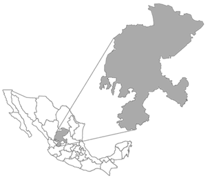
Table 1: Network of weather stations located within the territory of Mexican Zacatecas state.
| Station | Station name | Latitude | Longitude | Elevation (m) |
|---|---|---|---|---|
| 1 | Agua Nueva | 23° 46' 55'' | 102° 09' 39'' | 1932 |
| 2 | Calera | 22° 54' 00'' | 102° 39' 00'' | 2192 |
| 3 | Chalchihuites | 23° 14' 27'' | 102° 34' 31'' | 2060 |
| 4 | Concepción del Oro | 24° 37' 16'' | 101° 23' 26'' | 1940 |
| 5 | El Cazadero | 23° 41' 35'' | 103° 26' 50'' | 1898 |
| 6 | El Platanito | 22° 36' 43'' | 104° 03' 05'' | 990 |
| 7 | Leobardo Reynoso | 23° 10' 46'' | 103° 12' 26'' | 2090 |
| 8 | Excamé III | 21° 38' 58'' | 103° 20' 23'' | 1740 |
| 9 | Fresnillo | 23° 10' 22'' | 102° 56' 26'' | 2195 |
| 10 | Gruñidora | 24° 16' 29'' | 101° 53' 05'' | 1825 |
| 11 | Jerez | 22° 38' 31'' | 103° 00' 05'' | 2098 |
| 12 | Jiménez del Teul | 23° 15' 18'' | 103° 47' 54'' | 1900 |
| 13 | Juchipila | 21° 23' 14'' | 103° 06' 53'' | 1270 |
| 14 | La Bufa | 22° 47' 00'' | 102° 34' 00'' | 2612 |
| 15 | La Florida | 22° 41' 10'' | 103° 36' 09'' | 1870 |
| 16 | La Villita | 21° 36' 08'' | 103° 20' 13'' | 1790 |
| 17 | Loreto | 22° 16' 40'' | 101° 59' 15'' | 2029 |
| 18 | Gral. Gpe. Victoria | 22° 23' 43'' | 101° 49' 52'' | 2183 |
| 19 | Nochistlán | 21° 21' 55'' | 103° 50' 32'' | 1850 |
| 20 | Ojocaliente | 22° 24' 38'' | 102° 16' 09'' | 2050 |
| 21 | Pinos | 22° 16' 54'' | 101° 34' 47'' | 2408 |
| 22 | El Chique | 22° 00' 00'' | 102° 53' 23'' | 1620 |
| 23 | San Pedro Piedra Gorda | 22° 27' 09'' | 102° 20' 49'' | 2032 |
| 24 | Santa Rosa | 22° 55' 34'' | 103° 06' 47'' | 2240 |
| 25 | Teul de González | 21° 27' 42'' | 103° 27' 59'' | 1900 |
| 26 | Tlaltenango | 21° 46' 54'' | 103° 17' 45'' | 1700 |
| 27 | Trancoso | 22° 44' 39'' | 102° 22' 10'' | 2190 |
| 28 | Villa de Cos | 23° 17' 26'' | 102° 20' 44'' | 2050 |
| 29 | Villa García | 22° 10' 10'' | 101° 57' 27'' | 2120 |
| 30 | Villanueva | 22° 21' 43'' | 102° 53' 22'' | 1920 |
| 31 | Zacatecas | 22° 45' 39'' | 102° 34' 30'' | 2485 |
Cluster Analysis
Cluster analysis is an effective statistical tool to find homogeneous climate regions based upon observed values of meteorological variables (Unal et al., 2003; Karmalkar et al., 2011). This approach groups data objects based only on information found in the data that describes the objects and their relationships. The goal is that the objects within a group be similar to one another and different from the objects in other groups (Tan et al., 2007). The greater the similarity within a group and the greater the difference between groups, better or more distinct the clustering (Tan et al., 2007). In this research, we used a tree clustering algorithm to join objects (i.e.: monthly precipitation time series) into successively larger clusters (i.e.: regions under the basis of similar precipitation behaviors); the Canberra distance was used as linkage criteria and the Ward’s method was used as linkage rule.
The joining or tree clustering method uses the dissimilarities or distances between objects when creating the clusters. Distance is a measure of how close one record is to another. The distances can be based on a single dimension or multiple dimensions, with each dimension representing a rule or condition for grouping objects. On the other hand, dissimilarities are a set of rules to measure how close one cluster is to another. The Ward’s method is generally regarded as very efficient; however, it tends to create clusters of small size (Unal et al., 2003) and uses an analysis of variance approach to evaluate the dissimilarities between clusters. For the Ward’s method, the proximity or distance between two clusters is def ined as the increase in the squared error that results when two clusters are merged (Tan et al., 2007).
In this research, cluster analysis was performed by means of the R system version 3.4.4 (R Core Team, 2018) and hclust (R Core Team, 2018) and ape (Paradis and Schliep, 2018) packages. Both the R system and the packages are freely available at the Comprehensive R Archive Network (https://www.cran.r-project.org/).
Standardized Precipitation Index Estimation Model
The Standardized Precipitation Index (SPI) developed by McKee et al. (1993) is the number of standard deviations that observed cumulative precipitation deviates from the climatic average. The SPI was developed primarily for defining and monitoring drought. Following Komlan et al. (2017), the SPI is calculated through the following steps:
Monthly rainfall data is fitted to a gamma distribution whose probability density function is defined as:
for x >0.
Where g(x) is the probability density function, α is the shape parameter (α > 0), β is a scale parameter (β > 0), and
Where Γ(α) is the gamma function.
The parameters α and β are estimated as follows:
Where n is the number of precipitation observations and is the arithmetic mean over the time scale of interest. A cumulative probability G(x) of an observed amount of rainfall in a given month and time scale (if α and β estimators where used to integrate the probability density function with respect to x) is obtained as follows:
Substituting t for in the previous equation, results in the incomplete gamma function:
Nevertheless, the gamma distribution function is undefined for x = 0 and q = P(x = 0) > 0; where P(x = 0) is the probability of zero precipitation. Hence, the actual probability of non-exceedance H (x) should be calculated as follows (Edwards and McKee, 1997; Usman et al., 2014):
Where H(x) is the actual probability of non-excess and q the probability of x = 0. If m is zero in a sample of size n, then q is estimated as:
Finally, to calculate the SPI, the cumulative probability distribution H (x) is transformed into a standard normal variable Z with mean equal to zero and variance equal to one. The interpretation of wet or dry periods considering the SPI results were performed as stated by Hayes (2000) and the WMO (2012).
Several time scales are used for the computation of SPI on which changes in precipitation can affect different aspects of the water cycle (Komlan et al., 2017). In this study, we evaluated the SPI at timescales of 6 and 12 months. In fact, whereas the 6-month SPI describes droughts that affect plant life and agriculture (agricultural drought), the 12-month SPI refers to hydrological droughts, as pointed out by Bonaccorso et al. (2003). Due to the complexity to manually calculate the SPI, several computer programs have been developed for this purpose. One of the most used programs is the one developed by the United States National Drought Mitigation Centre. The program is freely available at http://drought.unl.edu/droughtmonitoring/SPI/SPIProgram.aspx. Nevertheless, in this research we used the R system version 3.4.4 (R Core Team, 2018) and SPEI (Beguería and Vicente-Serrano, 2013) and the packages ‘spei’ (Beguería and Vicente-Serrano, 2013) and ‘spi’ (Neves, 2012) for SPI’s estimation. These packages are freely available at the Comprehensive R Archive Network (https://www.cran.r-project.org/). In this study, regional monthly precipitation time series were used to compute the SPI values considering the results previously yielded by the clustering procedure.
Trends Estimation
SPI trends estimation was performed through the Mann-Kendall trend test. This approach is a nonparametric technique which calculates the τ (tau) value of Kendall (Mann, 1945; Kendall, 1975). It is based on the ranks of the data rather than individual values, which is considered robust even when there are outliers in the series.
Seasonal Mann-Kendall test. Given a set of x data observations sampled over n years, where there are m seasons per year such that X is given by:
In each regional time series, we tested the following null hypothesis, Ho: There is no trend in the series.
Following Hirsch et al. (1982), the seasonal Mann-Kendall test is:
Where
and
The values of S g and var(S g ) are used to compute the Z test value
Kendall’s tau statistic for the g-th season (τg) is defined as:
Finally, the Mann-Kendall test statistic (S’) is defined as:
Theil-Sen trend estimator. The Theil-Sen trend estimator (Sen, 1968; Theil, 1992) is robust for a linear trend in the time series with n values of x and using all the slopes between all data pairs:
Where j > k.
In this study, the R system version 3.4.4 (R Core Team, 2018) was used to calculate the Mann-Kendall S value, Kendall’s Tau and Sen’s slope estimator. For this purpose, we used the package rkt version 1.5 (Marchetto, 2017). Such a package is freely available at the Comprehensive R Archive Network (https://www.cran.r-project.org/).
RESULTS AND DISCUSSION
As pointed out ut supra, a cluster analysis was performed using 31 profiles of monthly precipitation with the aim of grouping them into successively larger groups (i.e.: Regional monthly precipitation time series). The dendrogram (Figure 2) revealed four clusters or regions: I, Semi-desert region (3 out of 31 profiles); II, Highlands region (14 out of 31 profiles), III, Mountains region (7 out of 31 profiles) and IV Canyons region (7 out of 31 profiles).
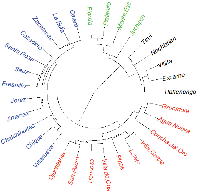
Figure 2: Radial dendrogram for 31 monthly precipitation time series through the Zacatecas state territory using amalgamation rule of Ward’s method and Canberra distance as linkage rule. Cluster I: (Black), Cluster II: (Green), Cluster III: (Blue) and Cluster IV: (Red).
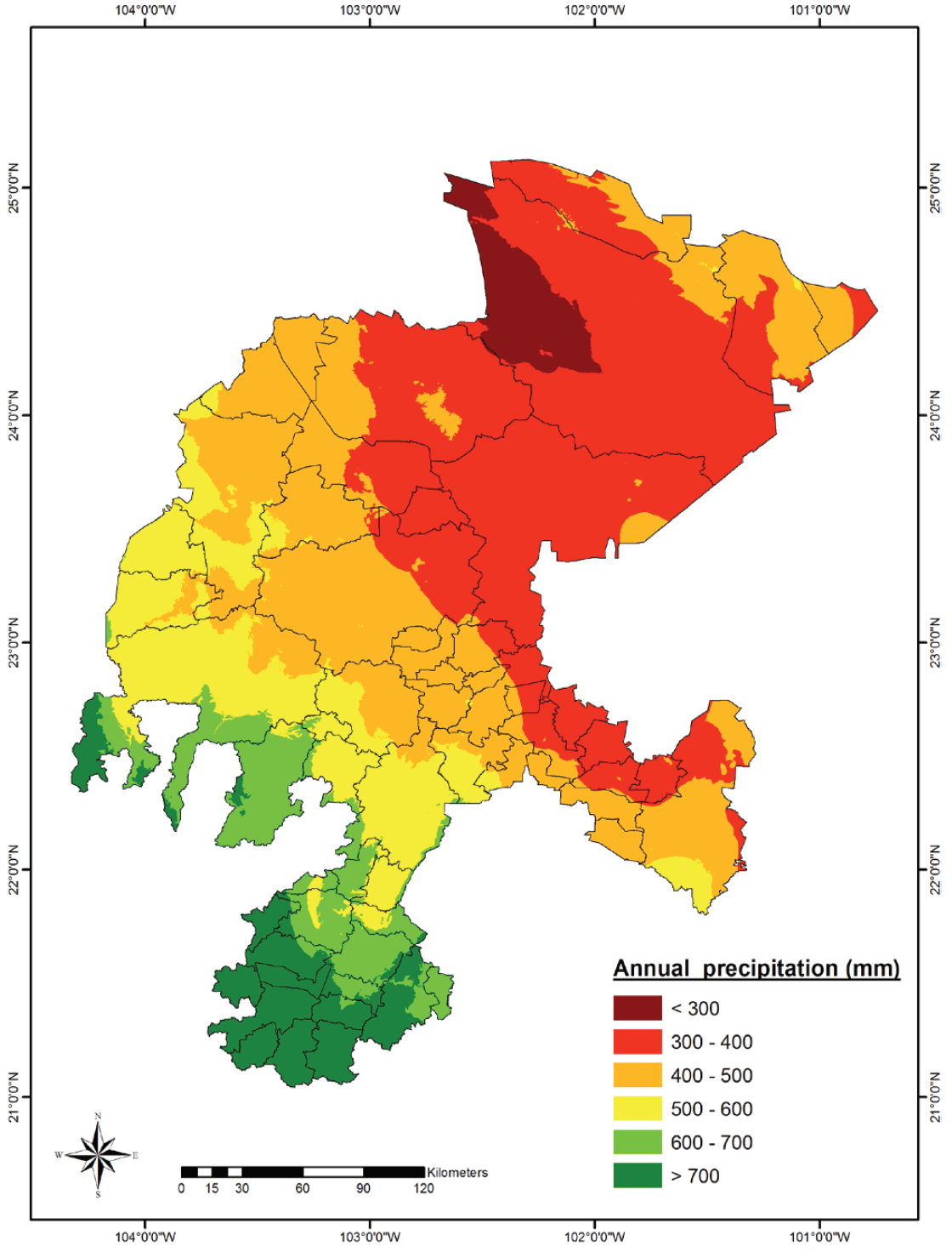
As expected, cluster analysis results agree with the spatial distribution of the annual mean precipitation throughout the Zacatecas state territory (Figure 3). Thus, the cluster I includes time series from weather stations with annual precipitation from 300 to 400 mm, the cluster II includes time series from stations with annual precipitation from 400 to 500 mm, the cluster III includes time series from stations with annual precipitation from 500 to 600 mm and the cluster IV includes time series from stations with annual precipitation > 700 mm.
Notably, the Ward’s method as linkage rule and the Canberra distance as linkage criteria allowed us to join monthly precipitation time series into successively larger clusters (i.e.: regions under the basis of similar precipitation behaviors). Then, we were able to identify four homogeneous regions under the basis of sites with similar rainfall regimes throughout the Mexico’s state of Zacatecas. Notably, our results agree with the spatial distribution of the annual mean precipitation along the state territory.
These results clearly suggest the Semi-desert region includes time series from weather stations with annual precipitation from 300 to 400 mm; the Highlands region involves profiles from stations with yearly rainfall from 400 to 500 mm; the Mountains region includes time series from sites with annual precipitation from 500 to 600 mm; and the Canyons region involves profiles from stations with yearly rainfall > 700 mm.
These rainfall patterns define the productive activities performed by inhabitants of each region. These activities represent important economic income to most of the families settled along the Zacatecas territory. In the Semi-desert region, goats are kept for dairy and meat production although those activities represent only low incomes at familiar level; the major production systems are characterized by small flocks (<100 animals), feeding based on grazing and browsing native vegetation, following regular routes and keeping the animals overnight in rudimentary shelters; the main products of these systems are veal kids (‘cabritos’) and culled goats (Tovar-Luna, 2009). In the Highlands region, the main crop is dry beans (Phaseolus vulgaris L.), followed by species for forage such as corn (Zea mays L.) and oat (Avena sativa L.), and horticultural species as pepper (Capsicum annuum L.), onion (Allium cepa L.) and garlic (Allium sativum L.). In the Mountains region, the main crops are dry beans (Phaseolus vulgaris L.) and corn (Zea mays L.), and people also practice forestry activities. In the Canyons region, the main activity refers to the cow-calf production system, production of guava (Psidium guajava L.), agave (Agave tequilana Weber) and a great variety of vegetables and flowers.
Standardized Precipitation Index
As mentioned previously, the members of each cluster allowed us to define four regional precipitation time series with the aim of compute their corresponding regional Standardized Precipitation Index (SPI) time series at 6-month and 12-month time scales useful to identify wet and dry episodes.
SPI at 6-month scale behavior. Results for the SPI for 6-month time scale are shown in Figures 4-7. In all the four regions, the rainy seasons from June to October is well defined. Those results disagree with the Bautista-Capetillo et al. (2016) statement about rainy season starts in April each year along the whole state territory. On the other hand, results strongly suggest dry season start in November and end in May.
The SPI values of the region I vary from -1 to 2.5 (Figure 4). Most of the rainy seasons were moderately wet with a few very wet, especially in the periods 1964-1968, 1970-1971, 1974-1976, 1978, 1980, 1989-1991, 2001-2003, 2007-2010 and 2012-2013. Notably, January 1992 was moderately wet. On the other hand, most of the winters were moderately dry. Nonetheless, November and December 1976 were moderately wet.
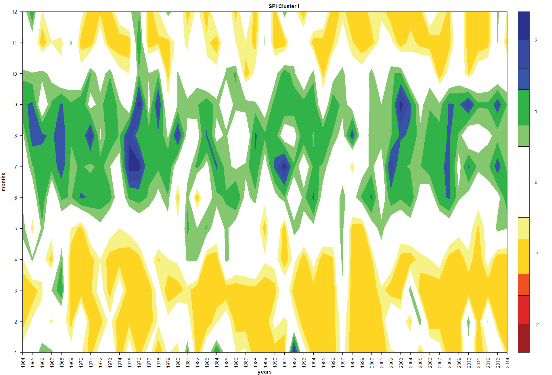
Figure 4: Standardized Precipitation Index at 6-month time scale in the Zacatecas (Cluster I, Semi-desert region) state of Mexico for the period of 1964-2014.
The SPI of region II varies from -1.5 to 2.5 (Figure 5). Most of the summer rainy seasons were moderately wet. Particularly, very wet summers are appreciated for the periods 1964-1967, 1969-1977, 1982-1991, 1993-1995, 1998, 2001-2004, 2006-2009 and 2012-2013. On the contrary, most of the winters were moderately dry. However, March 1967, November and December 1976, January 1976, and October-December 2013 were moderately wet.
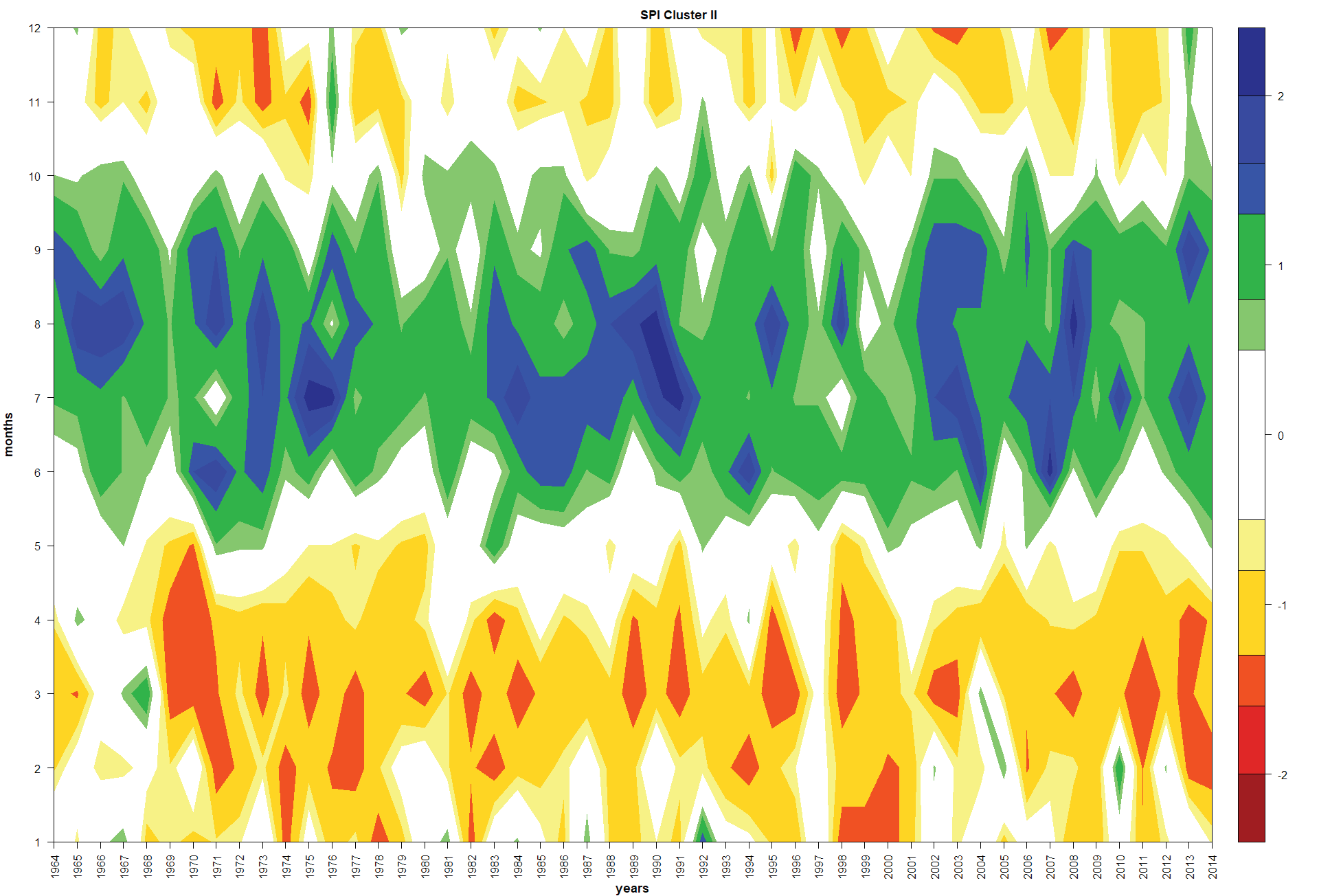
Figure 5: Standardized Precipitation Index at 6-month time scale in the Zacatecas (Cluster II, Highlands region) state of Mexico for the period of 1964-2014.
The SPI of the region III ranged from -1 to 2.5 (Figure 6). Most of the summers were very wet; those episodes occurred in 1964-1968, 1970-1977, 1983-1991, 1994-1995, 2002-2008 and 2012-2013. Remaining summer seasons were moderately wet. On the other hand, most of the winters were moderately dry; however, November and December 1976, October-December 1982, and October-December 2013 were moderately wet, whereas January 1992 was very wet.
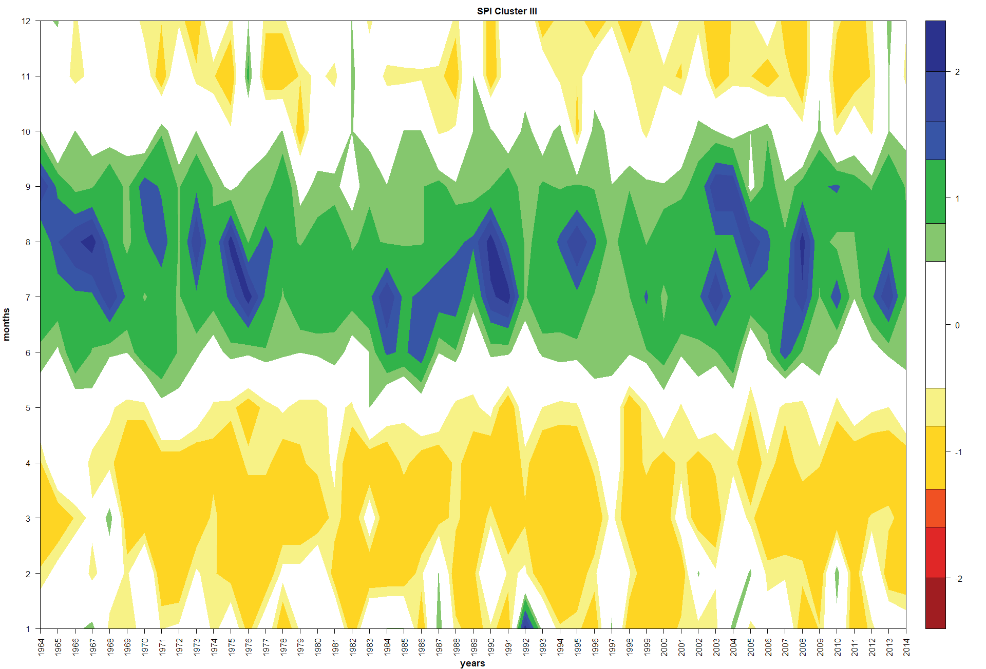
Figure 6: Standardized Precipitation Index at 6-month time scale in the Zacatecas (Cluster III, Mountains region) state of Mexico for the period of 1964-2014.
The SPI values of the region IV varied in the range of -1.5 to 2.5 (Figure 7). Most of the summers were very wet: 1964-1971, 1973-1996, 1998, 2000, 2002-2008, 2010, and 2013-2014. Remaining summers were moderately wet. On the contrary, most of the winters were moderately dry; nonetheless, January 1992 was very wet and October, November and December 2013 were moderately wet.

Figure 7: Standardized Precipitation Index at 6-month time scale in the Zacatecas (Cluster III, Canyons region) state of Mexico for the period of 1964-2014.
Different conditions in the four regions along the 50 years were clearly noted. In the Semi-desert and Highlands regions when SPI at 6-month scale was involved, most of the summer rainy seasons were moderately wet; however, in the cases of the Mountains and Canyons regions, most of the summers were very wet. On the other hand, most of the winters were moderately dry in all the four regions; however, several winter months were moderately and very wet depending on the region. For instance, November and December 1976 were moderately wet in the Semi-desert, Highlands and Mountains regions; in addition, October-December 2013 were moderately wet in the Highland, Mountains and Canyons region, and January 1992 was very wet in the Mountains and Canyons regions.
SPI at 12-month time scale Sen’s trends. Results of SPI at 12-month time scale are shown in Tables 2, 3 and 4. Notably, near normal months prevail in all four regions; that is, 431, 405, 415 and 420 normal months occurred in the semi-desert, Highlands, Mountains and Canyons regions, respectively. Nonetheless, wet and dry months were important issues. Number of wet months was higher than that of dry months in the cases of Semi-desert, Highlands and Canyons regions. On the other hand, number of wet months (81) was lower than that of dry months (105) in the Mountains region.
Table 2: Number of months (1964-2014) per region for each climate class according to the SPI values as proposed by Hayes (2000) and the WMO (2012).
| SPI | Class | Cluster/Region | |||
|---|---|---|---|---|---|
| I/Semi-desert | II/Highlands | III/Mountains | IV/Canyons | ||
| >2.0 | Extremely wet | 15 | 18 | 14 | 13 |
| 1.5 - 1.99 | Very wet | 14 | 25 | 22 | 29 |
| 1.0 - 1.49 | Moderately wet | 64 | 56 | 45 | 66 |
| -0.99 - 0.99 | Near normal | 431 | 405 | 415 | 420 |
| -1.0 - -1.49 | Moderate dry | 33 | 69 | 70 | 39 |
| -1.5 - -1.99 | Severely dry | 20 | 22 | 28 | 20 |
| ≤-2.0 | Extremely dry | 24 | 6 | 7 | 14 |
Table 3: Number of wet and dry months for different regions of Zacatecas state during the period 1964-2014.
| Cluster/Region | Number of months | Percentage of occurrence | ||||
|---|---|---|---|---|---|---|
| Wet | Normal | Dry | Wet | Normal | Dry | |
| I/Semi-desert | 93 | 431 | 77 | 15.47 | 71.71 | 12.81 |
| II/Highlands | 99 | 405 | 97 | 16.47 | 67.39 | 16.14 |
| III/Mountains | 81 | 415 | 105 | 13.48 | 69.05 | 17.47 |
| IV/Canyons | 108 | 420 | 73 | 17.97 | 69.88 | 12.15 |
All four regional SPI time series Sen’s trends were negative for the period 1964-2014 (Table 4). These trends were significant (P < 0.05) in the cases of wet and dry seasons, and annual period in the Semi-desert and Canyons regions, and in the annual period in the Mountains region. Notably, all trends were non-significant in the Highlands region although they were also negative. Nonetheless, those results indicate monthly SPI values are decreasing over time mainly in the Semi-desert and Canyons regions.
Table 4: Estimators of Mann-Kendall trend test and significant Sen’s slope for the monthly SPI series at the Zacatecas state, México.
| Cluster/Region | Season | Mann-Kendall S’ | Kendall’s τg | P value | Sen’s slope |
|---|---|---|---|---|---|
| I/Semi-desert | Wet | -3270 | -0.164 | 0.001 | -0.017 |
| Dry | -13658 | -0.170 | <0.0001 | -0.018 | |
| Annual | -30434 | -0.1694 | <0.0001 | -0.0174 | |
| II/Highlands | Wet | -944 | -0.047 | 0.319 | -0.005 |
| Dry | -3000 | -0.037 | 0.263 | -0.004 | |
| Annual | -7086 | -0.0394 | 0.1486 | -0.0043 | |
| III/Mountains | Wet | -1350 | -0.068 | 0.154 | -0.007 |
| Dry | -4331 | -0.054 | 0.106 | -0.005 | |
| Annual | -10196 | -0.0567 | 0.0377 | -0.0060 | |
| IV/Canyons | Wet | -2766 | -0.139 | 0.003 | -0.015 |
| Dry | -9271 | -0.016 | 0.001 | -0.012 | |
| Annual | -22442 | -0.1249 | <0.0001 | -0.0113 |
Note: Sen’s slope values in bold are significant at P < 0.05.
When SPI at 12-month scale was involved, number of wet months was slightly higher than dry months in the Semi-desert and Canyons regions. In the Highlands region, number of wet months was almost equal than number of dry months. In the Mountains region, number of wet months was slightly lower than dry months.
Markedly, results suggest decreasing SPI at 12-month scale trends during the last 50 years along the entire Zacatecas territory. In other words, results are compelling evidences on occurrence of weaker wet and heavier dry periods in all four regions but mainly in the Semi-desert and Canyons regions, where strongly occurred more extremely dry months. In fact, results indicate SPI values strongly decrease for wet and dry seasons in both regions and for annual period in the Semi-desert, Canyons and Mountains regions.
Decreasing SPI at 12-month scale trends imply prevail of negative values at the end of the study period (1964-2014) and indicate less than median precipitation. Therefore, all SPI trends, significant or not, were probably tied to unusual stream flows, reservoir levels, and groundwater levels as pointed out by Hayes (2000) and WMO (2012). In fact, in the Zacatecas state, most of its cultivated land has a rainfed agriculture and its aquifers are over-exploited with a deficit of about 201.1×10⁶ m3 per year (SEMARNAT, 2008). Thus, the evidenced trends may be having influence on the availability of surface water, groundwater levels and aquifers recharge in the near future throughout the entire Mexico’s state of Zacatecas. So, it is imperative to adjust inhabitants’ activities according to design planned climate change adaptation strategies.
Future research works should include SPI at 1-, 3-, 6-, 9-, 12-, and 24-month scales to generate knowledge on meteorological, agricultural and hydrological droughts at local level. Those studies should de focused on the type of SPI trends (increasing or decreasing monotonic and non-monotonic) useful to design adaptation strategies for drought-prone areas. SPI trends can be evidenced through the innovative Sen’s method, as pointed out by Yilmaz (2019). Moreover, other future works should use our strategy concerning splitting state territory in regional areas with different agricultural uses to carry out correlation analysis between SPI values and corresponding regional yields or El Niño Southern Oscillation Index values or fluviometric levels or water reservoir levels or piezometric levels (for instance, see Sobral et al.,2019).
CONCLUSIONS
Precipitation time series of each identified region allowed us to define four regional precipitation time series. We used those profiles to estimate their corresponding regional Standardized Precipitation Index (SPI) time series at 6- and 12- month time scales. The regional SPI time series proved to be effective to diagnose wet or dry periods at regional levels. Clearly, SPI results demonstrated rainy season may start at June and end at October most of years. On the other hand, results strongly suggest dry season might start in November and end in May most of years.

