texto en
  Inglés (pdf)
 Artículo en XML
 Referencias del artículo
 Enviar artículo por email
 Citado por SciELO
  Similares en
SciELO
Similares en
SciELO 
 Permalink
Introduction
In northwestern Mexico, the Baja California Peninsula (BCP) separates the Pacific Ocean from the Gulf of California (GC), a semi-enclosed sea that is bounded by the coastline of 4 northwestern states: Baja California, Baja California Sur, Sonora, and Sinaloa (Fig. 1). On the west coast of the BCP, the main forcing agent of the large-scale ocean dynamics is the California Current, a current that flows from north to south and parallel to the BCP and is characterized by low salinities and low temperatures (Lynn and Simpson 1987, Torres-Orozco 1993). In this zone, intense wind-driven upwelling events occur from April to June as a result of the Ekman transport generated by the trade winds that blow parallel to the BCP (Zaytsev et al. 2003).

Figure 1 Bathymetry of the entrance to the Gulf of California (in meters). Black dots are the locations of CTD casts used to fit the final generalized additive mixed model. Continuous line depicts the 200-m isobath. Broken line shows the division between the Pacific side (left) and the gulf side (right). The letters correspond to the locations of the randomly extracted CTD casts. The temperature profile that corresponds to each letter is shown in matching panels in Figure 9.
On the gulf (eastern) side of the BCP, water masses with high salinity and high temperature are predominant because the GC has a high evaporation rate and is considered an evaporation basin (Castro et al. 1994). At its southern extreme, the GC connects to the Pacific Ocean in a region known as the entrance to the GC; in this zone the cold, nutrient-rich California Current meets the warm, nutrient-poor Mexican Coastal Current (Kessler 2006) and an eddy train occurs as a product of the interaction between the Pacific Ocean forcing and the mainland topography (Zamudio et al. 2008). Because of these processes, strong thermal fronts occur in the area (Álvarez-Borrego 1983, Marín-Enríquez et al. 2018), making the entrance to the GC an interesting zone from the physical and the fisheries perspectives (Torres-Orozco et al. 2005).
Oceanographic cruises are campaigns designed mainly to collect data on seawater properties. Of those properties, water temperature has proven to be of main interest because it is a measure of the energy content in the ocean and most physical and ecological processes are closely linked to seasonal and year-to-year changes in water temperature. Additionally, recent studies have shown that the deeper oceans play a key role in regulating the Earth’s climate variability (Akbari et al. 2017), so assessing the ocean’s heat content at the subsurface levels is a very important endeavor.
Satellite-derived oceanographic data have been widely used in the different disciplines of marine science because it provides information that covers most of the world’s oceans at very fine spatiotemporal scales (Yang et al. 2013). Currently, the range of remote sensors is restricted to the surface of the ocean, and they cannot provide oceanographic data at subsurface levels (Fiedler 1988). The marine scientific community therefore relies on either direct observations or numerical modeling to obtain subsurface oceanographic data (Akbari et al. 2017). Several different modeling approaches have been used to estimate subsurface ocean temperature, including least squares; simple, multiple, and nonlinear regression; regression matrices; simple correlation; and interpolation. The reader can refer to Akbari et al. (2017) for a complete review on published works that deal with modeling subsurface ocean temperatures.
Nonlinear regression models are commonly used in a wide variety of scientific disciplines, such as fisheries ecology (Su et al. 2008, Zainuddin et al. 2008), health (Yang et al. 2012), and meteorology (Jones et al. 2013). Their use in the oceanography/hydrography disciplines, however, has been scarcely explored, and most published works rely on linear regression (Akbari et al. 2017). The papers by Richards et al. (2010) and Gómez-Ocampo et al. (2017) are of the few published works that used nonlinear regression models and oceanographic data. Using generalized additive models (GAMs) to monitor and standardize water quality parameters and oceanographic data for the coastal zone off Southeast Queensland, Australia, Richards et al. (2010) identified interesting nonlinear relationships between a coastal current and water turbidity, a finding with important implications in the operation of a desalination plant. The authors concluded that the application of GAMs in different research areas is “clearly evident” (Richards et al. 2010). Gómez-Ocampo et al. (2017) used GAMs to model surface chlorophyll concentration and primary productivity as a function of different environmental variables (absolute dynamic topography and Ekman pumping) and suggested that the GAMs produced a better fit when compared to other modeling approaches to predict chlorophyll and primary productivity.
The main objective of this paper is to explore nonlinear regression models as an alternative to the more complex deterministic models that are traditionally used to generate temperature profiles, and to assess how the temperature profiles predicted with nonlinear regression models deviate from in-situ observations and from profiles generated by hydrodynamic models. Here, it is shown that at least 90% of the variation of temperature profiles in the upper 200 m can be explained by a nonlinear regression model that includes variables as proxies of the mesoscale, seasonal, and interannual variation (sea surface dynamic topography); vertical water transport (wind stress curl); an interannual component (Oceanic Niño Index); a random term (month); and spatial (latitude, longitude) components. Although the results of the final nonlinear regression model presented here deviate from the in-situ observations and from the profiles generated using hydrodynamic models, the present paper could provide a baseline for scientific works that seek to use nonlinear regression to model different seawater properties, a research field that is virtually unexplored.
Materials and methods
Data
Temperature profile data were obtained from the Global Temperature and Salinity Profile Programme (GTSPP), available from the Environmental Research Division’s Data Access Program (ERDDAP) server of the US National Oceanic and Atmospheric Administration (NOAA) (Simmons 2017; dataset ID: erdGtsppBest). The dataset included day, month, year, longitude, latitude, temperature, and salinity for depths of 1 to 2,013 m, covering an area from -114.5º to -105.9º W and 15.5º to 25.8º N (Fig. 1) and a timeframe from June 2007 to November 2016. Only data for the first 200 m of the water column were used, because (1) that’s where most of the temperature vs. depth variation occurs (thermocline, mixed layer) (Fiedler and Talley 2006) and (2) most commercially important fisheries (tunas, sardines, billfish) occur within those depths, in the epipelagic zone (Holland et al. 1990, Emmett et al. 2005, Torres-Orozco et al. 2005).
A thorough exploratory analysis of the data was performed. A common issue with this type of dataset is that temperature is not measured in uniform depth intervals (probably due to different study designs or technical equipment differences). In the particular case of this dataset, depth intervals ranged from 1 to 42 m; of these, ~90% of temperature profiles were recorded in depth intervals of <10 m, and 36% in depth intervals of 1 m. Linear interpolation was performed to ensure that all profiles had Zmax - Zmin observations (i.e., a profile in which the conductivity, temperature, depth [CTD] sensor started to measure temperature at 5 m and ended at 195 m would have 195 - 5 = 190 observations after interpolation). Interpolating the database resulted in 127,595 temperature observations.
According to Godínez et al. (2010) the seasonal, interannual, and mesoscale dynamics are almost equally important to determinate the sea surface circulation in the study area (35%, 35%, and 30%, respectively). To account for seasonal variation, month was included as a random effects variable, and to account for year-to-year variability in temperature profiles, the Oceanic Niño Index (ONI) was used because the interannual variability of the circulation at the entrance to the GC is dominated by El Niño/Southern Oscillation (ENSO) (Godínez et al. 2010). ONI is calculated as the monthly anomaly of the sea surface temperature data from a rectangular area near the equator (5º S to 5º N and 120º to 170º W) known as El Niño 3.4 region. ONI data for the same period as the CTD database (2007-2017) were obtained from NOAA’s Climate Prediction Center (http://origin.cpc.ncep.noaa.gov/products/analysis_monitoring/ensostuff/ONI_v5.php).
On the other hand, the sea surface dynamic topography (SSDT) was used as a proxy to account for the mesoscale, interannual, and seasonal variability in the temperature vs. depth variation. Data for SSDT were obtained from the Copernicus Marine Environmental Monitoring Service (http://marine.copernicus.eu/) for the 2006-2017 period, with a monthly temporal resolution and a 0.08º × 0.08º spatial resolution. To account for the temperature vs. depth variation associated with vertical water transport, wind data were also extracted from Copernicus; the wind database had a monthly temporal resolution and a 0.25º spatial resolution. Including wind in regression-based models is not a trivial task, because (unlike temperature and SSDT) wind is a vector quantity. Because wind data were used as a proxy for vertical transport, the wind stress curl (WSC) was included as a predictor variable in the statistical modeling process. WSC was calculated from the wind data using the following equation:
where ∂τ y and ∂τ x are, respectively, the meridional and zonal changes of the wind stress τ, and ∂ x and ∂ y are the size of the pixels (0.25º) of the wind database.
Wind stress τ was calculated using the empirical equations proposed by Large and Pond (1981):
where C D is a dimensionless drag coefficient (1.2 × 10⁻³), ρ air is the density of air (1.22 kg·m-3), and U is the wind speed at 10 m above sea surface. WSC was calculated using the curl function of R’s oce package v.1.2-0 (Kelley and Richards 2017).
Because neither the nodes of the SSDT nor the wind grids exactly matched the coordinates of the CTD casts of the GTSPP database, the closest point of the SSDT and the wind grid to each CTD cast location (for the corresponding month/year when the CTD cast was carried out) was used as a proxy of SSDT and wind for each of the 656 locations of the CTD casts. This was accomplished by writing a function in the R environment that calculates the distances between the locations of each CTD cast and each of the nodes of the SSDT grid, and returns the coordinates of the grid that are closest to the location of each CTD cast.
Thermocline depth
Thermocline depth is one of the most important variables in hydrography because changes in this variable are responsible for numerous biological, physical, chemical, and ecological processes. In order to assess the model’s capacity to reproduce the temperature profiles, the thermocline depth of the observations and the predictions made by the model was calculated according to Fiedler and Talley (2006), who suggested that thermocline is the depth where the maximum value of dT/dZ occurs.
Statistical modeling
A generalized additive mixed model (GAMM) was used to model the relationship between temperature and depth, SSTD, WSC, latitude, longitude, and ONI. GAMMs are extensions of the classical linear regression model, but the 2 approaches differ by 3 main characteristics. First, unlike linear regression models, GAMMs can incorporate different error distributions (other than Gaussian). Second, GAMMs are capable of dealing with nonlinear relationships between the response and the independent variables in a semiparametric manner (Maunder and Punt 2004). The degree of “how nonlinear” the relationship is between the response variable and any covariate is quantified by the effective degrees of freedom (EDF), with EDF = 1 depicting a linear relationship and EDF > 1 depicting some degree of nonlinearity (Wood 2006). Third, GAMMs can incorporate a random effect component, which is useful when the heterogeneity of variances assumption is violated. The decision of using a gamma distribution for the error was based on the following: (1) the histogram of the response variable (temperature) was skewed to the left (non-normal appearance), (2) gamma distribution can be used for continuous positive variables (such as temperature), and (3) gamma distribution is capable of dealing with data with reasonable amount of spread at the expense of the estimation of an extra parameter (Zuur et al. 2009).
Because the oceanographic features that distribute the water masses in the study area are different on the Pacific and gulf sides of the BCP, a “Region” variable was nested in the model. “Region” is a categorical variable with 2 levels: gulf and Pacific. The division between the gulf and Pacific areas was made according to Lavín and Marinone (2003), who suggested that the gulf is separated from the Pacific Ocean by an imaginary line from Cabo San Lucas, in the BCP, to Cabo Corrientes, in the Mexican state of Jalisco (See Fig. 1). Nesting of the “Region” variable was accomplished by setting the argument of the gamm function of mgcv (Wood 2006) in R to “Region” (by = Region) (R Core Team 2016), ensuring that one curve was fitted for the profiles on either side of the study area (Wood 2006). The nested “Region” variable was included in all the predictor variables, with the exception of ONI, because ONI data can account only for temporal (not spatial) year-to-year variability.
To assess the relative importance of each variable, a stepwise modeling approach was used. In this approach, each single covariate is added at a time, and its degree of importance is assessed with the percentage of explained deviance. The decision on when to retain or drop a covariate from the GAMM was based on the Akaike information criterion (AIC), and any variable that resulted in a decrease of at least 2 units in the AIC was retained in the model (Burnham and Anderson 2002). When the effect of 2 variables together differs from the sum of their separate effects, using interaction terms is a useful approach (Wood 2006). The interaction term between longitude and latitude was included to account for the spatial setting, a procedure that is commonly used in spatially explicit statistical modeling (see, for example, Su et al. 2008 and Marín-Enríquez et al. 2018). A common problem in regression-based statistical models arises when 2 or more of the covariates are correlated to each other. To minimize the potential bias induced by multicollinearity, a concurvity analysis of the models was performed at each step of the stepwise process. Concurvity can be seen as a nonlinear extension of multicollinearity (Wood 2006) and takes values between 0 and 1, with 1 depicting perfect collinearity between any 2 covariates.
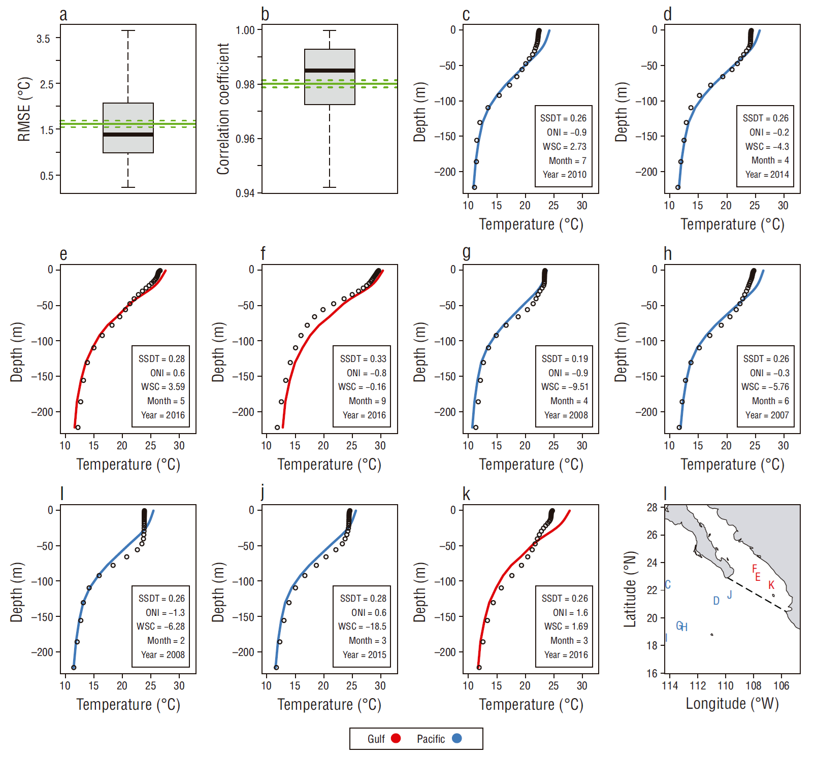
Model validation process was divided in 4 parts. First, normality and heterogeneity were assessed using standard analysis of the fitted model’s residuals (histogram of the residuals, scatterplots of residuals vs. independent variables). Second, the model’s potential overfitting and its predictive capacity were tested by applying the fitted model to an independent dataset (a dataset that was not used in the model-fitting process). Predicted vs. observed values for this last part were explored by calculating the root-mean-square error (RMSE) and the Pearson correlation coefficient of the observed vs. predicted temperature data and of the observed vs. predicted thermocline depth for all the profiles of the independent database. For this part, data for 2017 was extracted from the same website from where data used in the fitting process was extracted. Splitting of datasets and predictions made on independent datasets have proven to be a useful tool to assess model overfitting and predictive accuracy of statistical models (Martínez-Rincón et al. 2012, Farrell et al. 2014). Third, to assess possible bias in the final model due to the fact that processes that can regulate temperature profiles on each side of the BCP are somehow different, profiles from both the 2007-2016 (4 profiles for each side) and the 2017 (3 profiles for the gulf side and 2 profiles for the Pacific side) databases were randomly extracted from the database. Once the profiles were randomly chosen, the final GAMM was used to predict the corresponding longitude, latitude, SSDT, WSC, and ONI combinations for each of the extracted profiles. Results were explored visually, and the Pearson correlation coefficient was calculated for each of the randomly chosen profiles. Additionally, the differences in the thermocline depth between the model’s predictions and the observations were assessed using frequency histograms and by calculating linear correlation and RMSE for all the profiles of the 2017 database. Fourth, the results of the model were compared to the temperature profiles obtained from the hydrodynamic models. For this last part, temperature profile data were extracted from the Copernicus website (http://marine.copernicus.eu/), and the Pearson correlation coefficient and the RMSE were calculated to assess the differences between the predictions of the model and the profiles extracted from Copernicus. In order to evaluate the final GAMM’s performance with respect to the data obtained from the hydrodynamic models, the differences in thermocline depth between the model’s prediction and the Copernicus profiles were also assessed using frequency histograms (observed minus modeled thermocline depth for both the GAMM and the Copernicus data). The modeling process was carried out using the mgcv library v.1.8-22 (Wood 2006) of the R environment (R Core Team 2016).
Results
Observed spatial variability
Of the 656 temperature profiles, 545 (~83%) were carried out on the Pacific side and 111 (~17%) on the gulf side. Most of the profiles on the Pacific side took place during the first half of the year and most profiles on the gulf side took place during June-November, although the monthly distribution of the CTD casts was relatively well distributed across the year (Fig. 2).
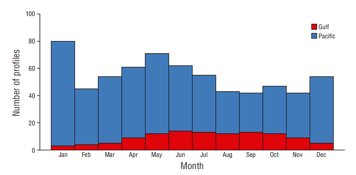
Figure 2 Monthly distribution of the CTD casts used to fit the final generalized additive mixed model, for the Pacific (blue bars) and gulf (red bars) sides.
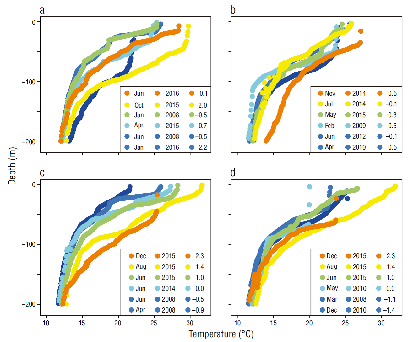
Figure 3 shows samples of temperature profiles carried out during different years, months, and El Niño conditions on the Pacific and the gulf sides. High temperatures (>25 ºC) were more common on the gulf side of the study area than on the Pacific side. Well-defined mixed layers of around 50 m thick were observed on the Pacific side when ONI conditions were low (approximately -0.8, February 2009) and high (~2.3, December 2015). Temperature values of ~20 ºC were observed for depths of ~75 m on the Pacific side, except during February 2009 and July 2014, when ONI values were approximately -0.1 to -0.6 and temperature values were noticeably low (Fig. 3b, d). On the gulf side, upper-layer temperatures of >25 ºC were observed during August/October 2015 and June 2016, when positive ENSO phases (ONI: ~0.1 to 2) occurred. Surface temperatures of ~30 ºC were observed on the gulf side during August and October 2015 (ONI: ~1.4 and 2, respectively). Well-defined mixed layers with a thickness of ~50 m were observed during positive ONI conditions (ONI: >2) in 2015 and 2016 (Fig. 3a, c). The deepest mixed layer on the gulf side (>100 m) was observed during January 2016, when ONI values were highest (~2.2) across the whole study period (Fig. 3a).
Statistical modeling
The final GAMM explained 86.2% of the total deviance. The validation process of the fitted GAMM was satisfactory: histogram of Pearson residuals appeared to be normal and centered approximately at zero, and no signs of residual heterogeneity were apparent for any of the covariates of the model (Fig. 4), except for the spatial distribution of the residuals. Although some clustering of the residuals was observed, no apparent spatial pattern was observed (Fig. 4f). Concurvity was low (<0.3) for all single covariates, which suggests low multicollinearity amongst predictors. All variables resulted in a decrease of at least 2 AIC units, and depth was the variable that had the higher explained deviance (69.1%). From the environmental variables, SSDT was the one that accounted for the higher explained deviance (14.3%) and highest decrease in AIC (75,067.07; Table 1).
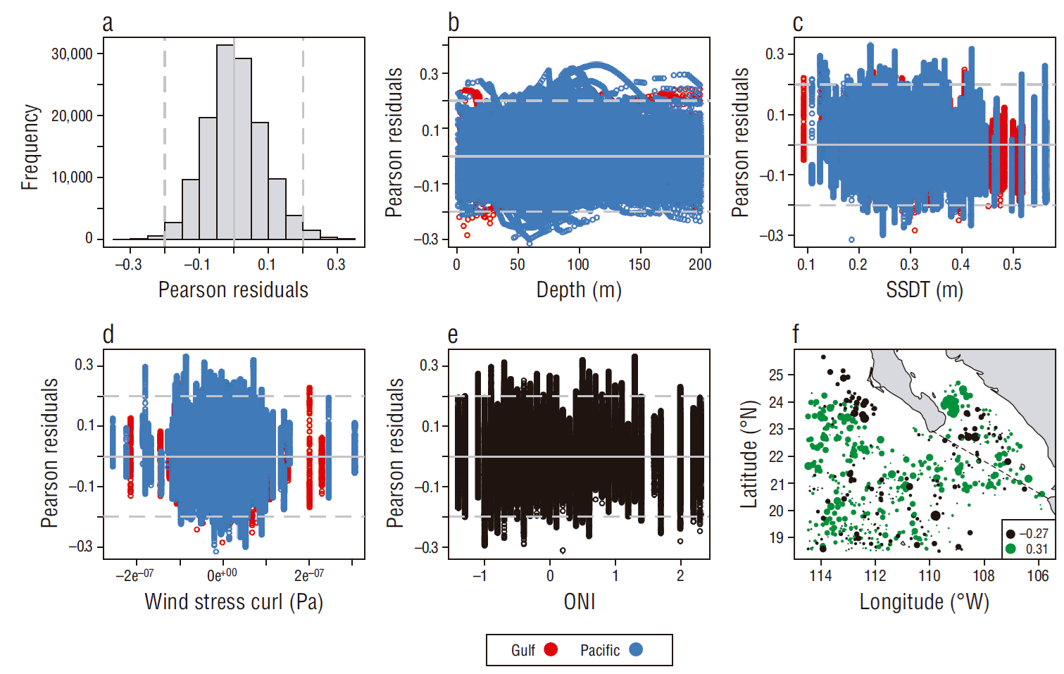
Figure 4 Diagnostic plots of the Pearson residuals of the final generalized additive mixed model: histogram of the fitted generalized additive mixed model (a) and residuals vs. depth (b), sea surface dynamic topography (SSDT) (c), wind stress curl (d), Oceanic Niño Index (ONI) (e), and longitude/latitude (f). Continuous gray line is the theoretical mean (zero), and broken gray lines depict the -0.2, 0.2 quantile interval. Broken black line in f marks the division between the Pacific side and the gulf side.
Table 1 Summary of the final generalized additive mixed model fitted to temperature profiles obtained from CTD casts from June 2007 through November 2016 in the Pacific Ocean off Mexico. The final explained deviance is depicted in bold.
| Variable | Region | EDF | Explained deviance (%) | Cumulative deviance (%) | AIC | |DAIC| |
| Temp ~ α + s(Depth) | Depth(by=G) | 8.54 | 69.10 | 69.10 | -189,361.8 | - |
| Depth(by=P) | 8.58 | |||||
| Temp ~ α + s(Depth) + s(SSDT) | SSDT(by=G) | 8.08 | 14.92 | 83.40 | -264,428.9 | 75,067.07 |
| SSDT(by=P) | 8.93 | |||||
| Temp ~ α + s(Depth) + s(SSDT) + s(WSC) | WSC(by=G) | 8.89 | 0.40 | 83.80 | -266,547.6 | 2,118.71 |
| WSC(by=P) | 8.90 | |||||
| Temp ~ α+ s(Depth) + s(SSDT) + s(WSC) + s(ONI) | - | 8.91 | 0.30 | 84.91 | -267,756.5 | 1,208.92 |
| Temp ~ α + s(Depth) + s(SSDT) + s(WSC) + s(ONI) + s(Lon,Lat) | - | 28.85 | 2.00 | 86.10 | -285,869.1 | 18,112.50 |
| Temp ~ α + s(depth) + s(SSDT) + s(WSC) + s(ONI) + s(Lon,Lat) + Region | - | - | 0.10 | 86.20 | -286,285.5 | 416.30 |
EDF, effective degrees of freedom; AIC, Akaike information criterion; Temp, temperature; SSDT, sea surface dynamic topography; WSC, wind stress curl; ONI, Oceanic Niño Index; Lon, longitude; Lat, latitude; G, gulf; P, Pacific.
The partial effects plots of the GAMM suggested that mean temperatures at the surface were higher on the gulf side (~29 ºC) than on the Pacific side (~25 ºC). The dT/dZ gradient appeared to be more abrupt for the mean profile of the gulf side, because differences of around 4 ºC between the profiles for the gulf and Pacific sides were observed at the surface, and differences <1 ºC were observed at around 50 m; additionally, temperature appeared to be higher on the gulf side throughout the whole water column (Fig. 5a). In general, higher temperatures were observed at higher SSDT values in both regions; higher mean temperatures (~22 ºC) were observed on the gulf side when SSTD values >0.5 m occurred. On the other hand, a peak of high mean temperature (~23 ºC) on the Pacific side agreed with SSTD values of ~0.48 m (Fig. 5b). The effect of WSC on mean temperature was mild for WSC values ranging from -1.5 × 10⁻⁷ to 1 × 10⁻⁷ Pa, when only slight variations around the temperature value of 18 ºC were observed. Low mean temperatures on the gulf (~16 ºC) side were associated with relatively high WSC values (2 × 10⁻⁷ Pa), and high temperatures (~29 ºC) were associated with WSC values > 2 × 10⁻⁷ Pa. For the Pacific side, low temperatures (~15 ºC) were also associated with relatively high WSC values (2 × 10⁻⁷ Pa). No WSC values >2.5 × 10⁻⁷ Pa were observed on the gulf side, which caused the effects plots to produce unrealistic values (Fig. 5c). As expected, high ONI values (~1.9 ºC) were associated with high mean temperatures (~18.8 ºC) (Fig. 5d). Spatially, higher mean temperatures were observed on the western and northwestern parts of the study area (inside the gulf), and lower temperatures were observed in the northeastern zone of the Pacific region (Fig. 5e). The parametric effect of the nested variable “Region” showed that mean temperatures were statistically higher on the gulf side when compared to the temperatures measured on the Pacific side (Fig. 5f).
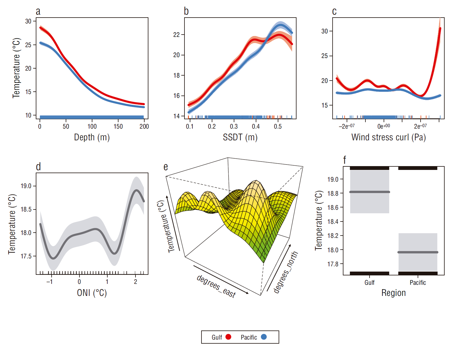
Figure 5 Partial effects plots of the predictor variables used in the final generalized additive mixed model: depth (a), sea surface dynamic topography (SSDT) (b), wind stress curl (c), Oceanic Niño Index (ONI) (d), latitude/longitude interaction (e), and mean parametric temperature for the Pacific and gulf sides of the study area (f). Shades in a-c depict the 95% Bayesian credibility interval, and lines perpendicular to the x-axis (rug plot) depict the density of the observations for each variable.
The model fitted to the 2007-2016 database was statistically satisfactory (correlation between observed and predicted temperature was ~0.93, P < 0.05, and the RMSE was ~1.55 ºC). However, important differences between in-situ and predicted thermocline depths were observed. For the gulf side of the study area, mean difference in thermocline depth was ~25.55 m (95% CI: ±7.01 m; SD = 37.37 m) and for the Pacific side mean difference was 37.92 m (95% CI: ±3.25 m; SD = 38.62 m), suggesting that the final GAMM underestimates thermocline depth (Fig. 6). Correlation between observed and modeled thermocline depths was low (0.21) and significant (P < 0.05). For the gulf side of the study area, higher deviations (~50 m) were observed during June 2014 and July 2015, and deviations of ~0 m were present during April through July 2008. For the Pacific side, higher deviations (>100 m) were observed during July through September 2011 and October/December 2015, and lower deviations (<20 m) were mainly observed during the second half of 2007 and during April through December 2012 (Fig. 7).
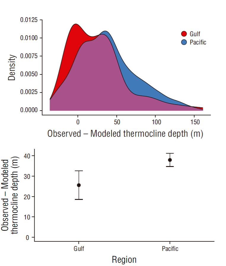
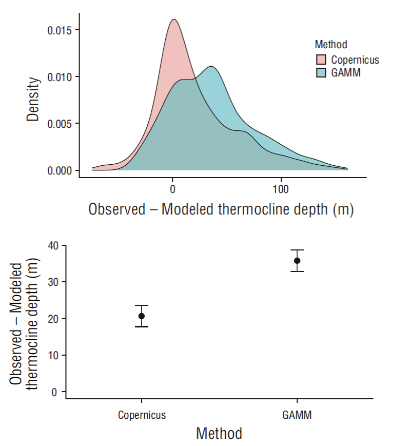
Figure 6 Deviations in the observed minus the modeled thermocline depths for the 2007-2016 data, which were used to fit the generalized additive mixed model. Kernel density curves (top) and mean deviations with 95% confidence intervals (bottom) for the Pacific and gulf sides of the study area.
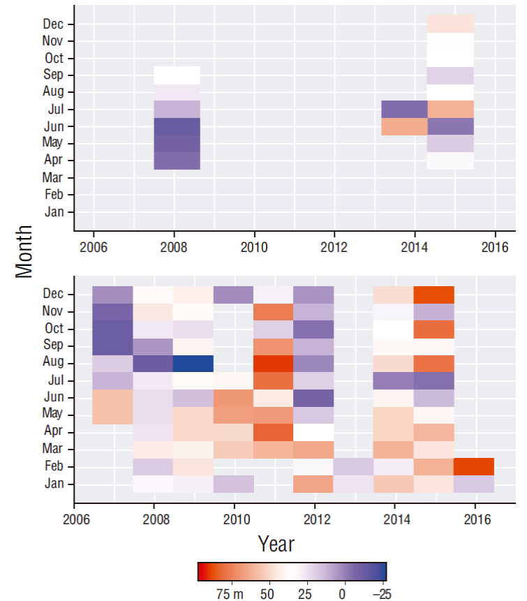
Figure 7 Hovmöller diagram of the mean monthly deviations of the observed minus the modeled thermocline depths for the gulf (top) and Pacific (bottom) sides of the study area. Color scale is in meters.
Although the model’s predictive performance based on an independent dataset (database of profiles for 2017) was also statistically satisfactory (predicted and observed temperatures were highly correlated [ρ ~0.93, P < 0.05] and the RMSE was ~1.48 ºC), some important deviations in observed vs. modeled thermocline depths were observed. For the gulf side, the mode for the difference in observed vs. modeled thermocline depths was around -10 m, and for the Pacific side it was around 22 m. Mean deviations for thermocline depth were 3.28 m (95% CI: ±9.800 m; SD = 22.68) for the gulf side and 18.40 m (95% CI: ±6.185 m; SD = 19.86 m) for Pacific side (Fig. 8). The correlation coefficient for the in-situ vs. modeled thermocline depths from the 2017 validation data was ~0.44, and it was statistically significant (P < 0.05).
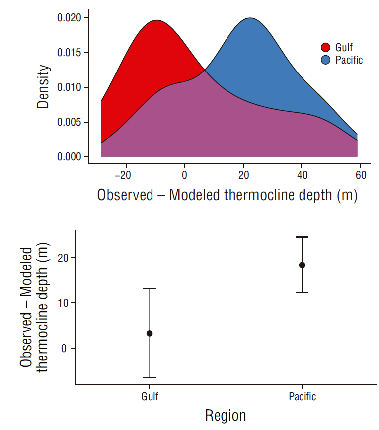
Figure 8 Deviations in observed minus the modeled thermocline depths for the 2017 data, which were used to validate the generalized additive mixed model. Kernel density curves (top) and mean deviations with 95% confidence intervals (bottom) for the Pacific and gulf sides of the study area.
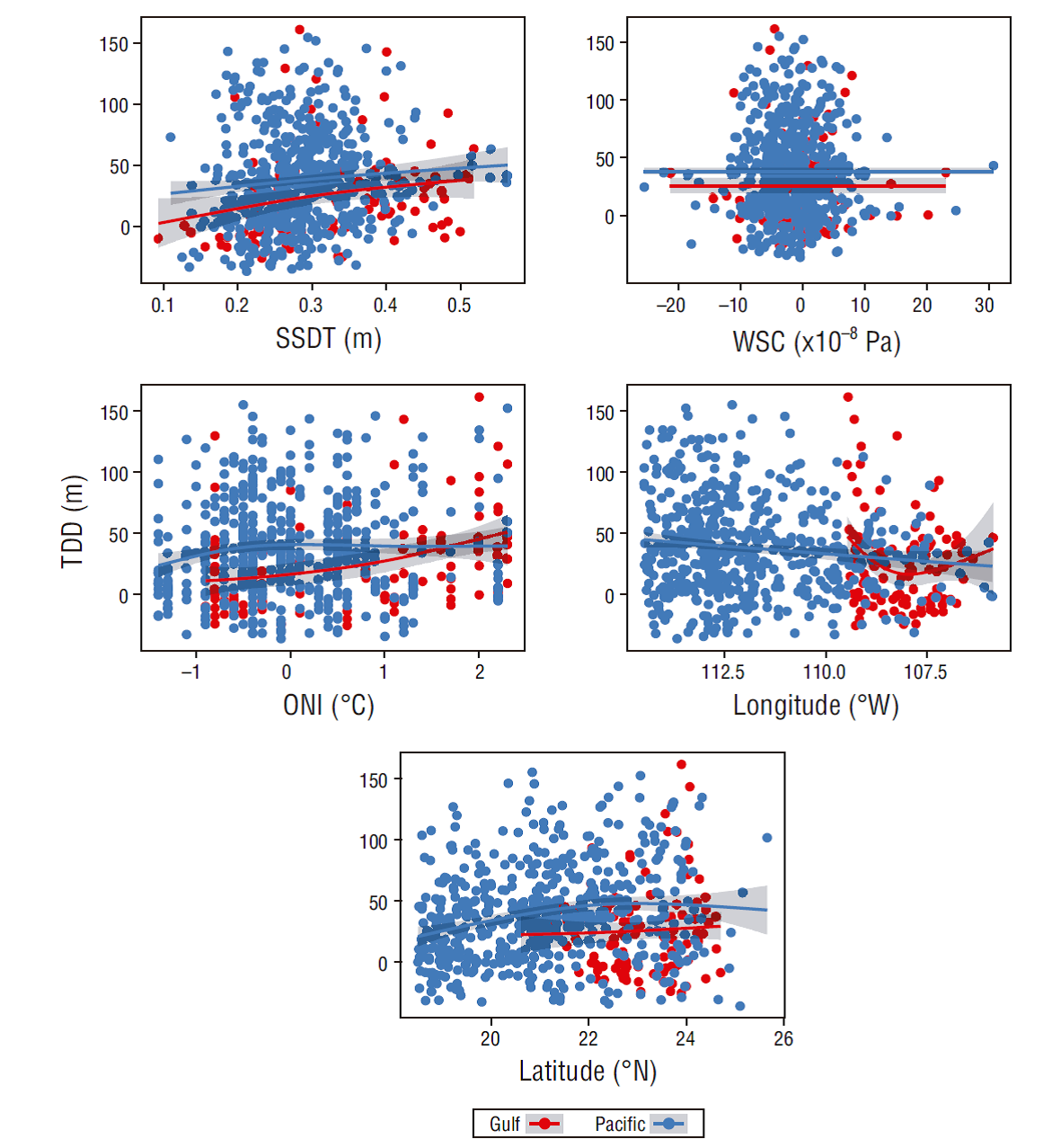
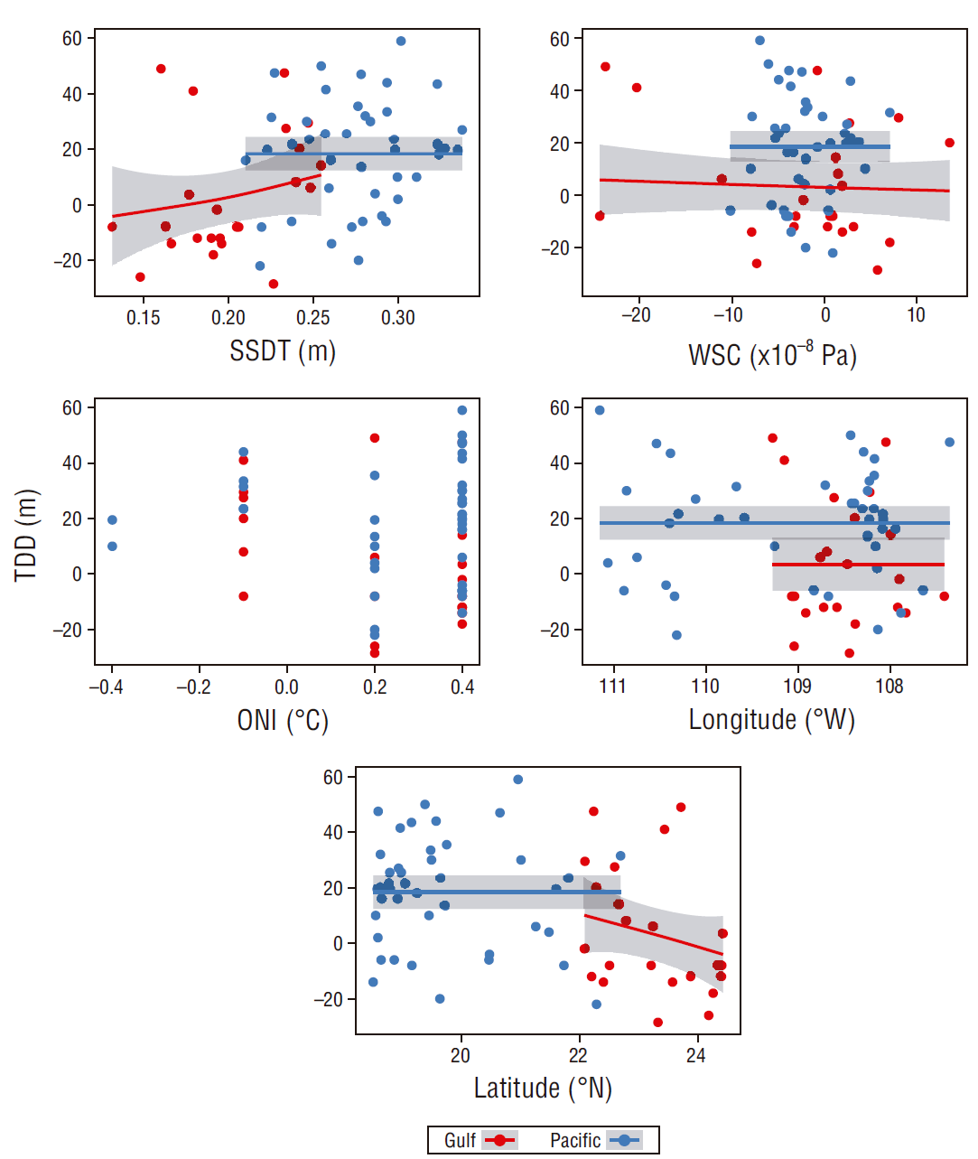
In general, deviations between observed and modeled thermocline depths appeared to be larger for the Pacific side of the study area than for the gulf side. The larger deviations were associated with higher SSDT (>0.25 m) and positive ONI values, for both the training (2006-2016) and the validation (2017) datasets. A spatial effect was also apparent, because higher deviations were observed at around 22 ºN and west of 112.5 ºW for the training dataset and at around 22 ºN for the validation dataset. No apparent pattern was observed for WSC (Figs. S1, S2).
The observed and predicted temperature profiles that were randomly extracted from the Pacific and gulf datasets are presented in Figures 9 and 10. Deviations between observed and modeled temperatures of up to 2 ºC were observed in some of the profiles that were carried out during 2007-2016. The model apparently failed to reproduce the observed profiles when the mixed layer was more evident, although it reproduced the profiles for the gulf side reasonably well; for example, a deviation in observed vs. modeled thermocline depth of approximately -13 m was observed in a May 2016 profile (Fig. 9c, Table 2). That profile was carried out during mild SSDT conditions (~0.22 m), relatively high downward water transport (-1.08 × 10⁻⁸ Pa), and positive ONI conditions (0.6). Larger deviations were also observed in profiles for the gulf side (~42.21 m), although the model appeared to reproduce the observations well (Fig. 9d); mean environmental conditions when this CTD cast was carried out were mild downwelling (-1.96 × 10⁻⁸ Pa), mild SSDT (0.27 m), and neutral ONI (~0.0).
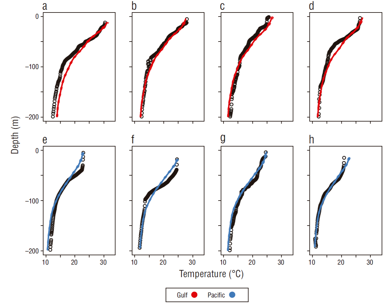
Figure 9 Observed (circles) and model-predicted (continuous line) temperature profiles that were randomly chosen for the gulf (red) (a-d) and Pacific (blue) (e-h) sides of the study area. Geographic location of each CTD cast is depicted in matching letters in Figure 1.
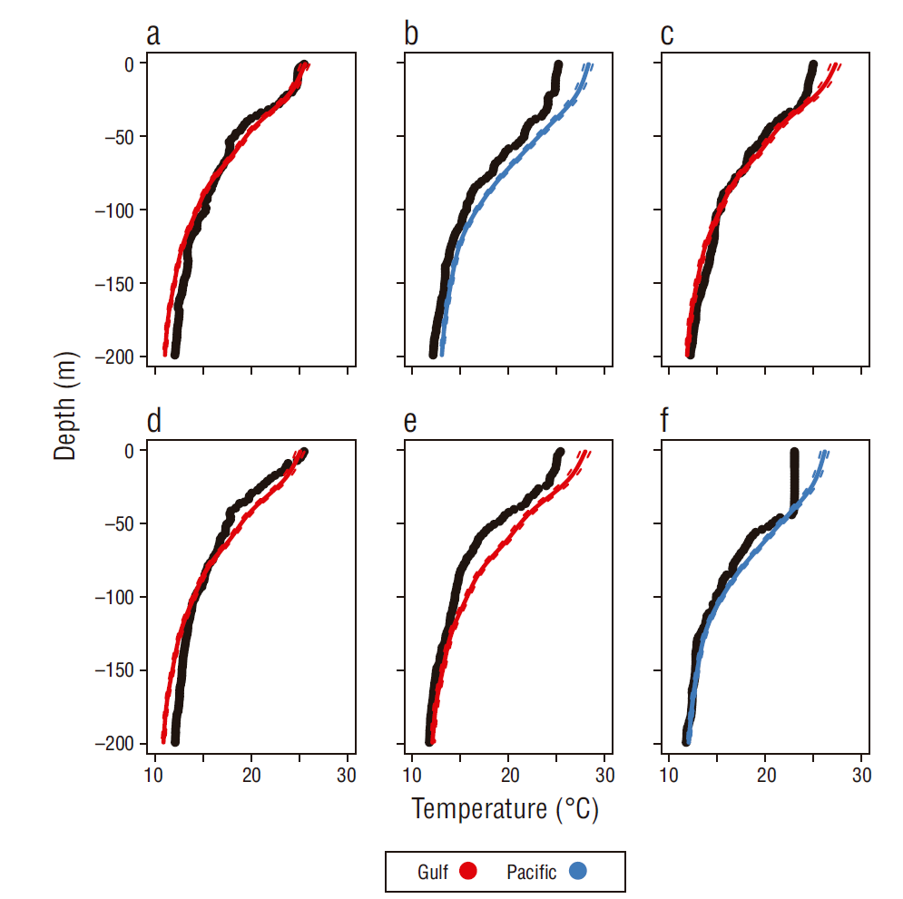
Figure 10 Observed (black dots) and model-predicted (continuous line) temperature profiles that were randomly extracted from the 2017 validation dataset for the Pacific (blue continuous line) and gulf (red continuous line) sides of the study area. The locations and the descriptive statistics of the profiles are shown in Table 3.
Table 2 Descriptive statistics for the profiles that were randomly chosen from the 2007-2016 database. The letters in the first column to the right match the panels displayed in Figure 9.
| Panel | Month | Year | Zmin (m) | Zmax (m) | Longitude | Latitude | SSDT (m) | WSC (×10-8 Pa) | ONI (ºC) | Zt observed (m) | Zt predicted (m) | Zt difference (m) | r |
| a | Sep | 2016 | 12 | 199 | -107.08 | 22.92 | 0.38 | -1.53 | -0.8 | 57.68 | 34.65 | 23.03 | 0.97 |
| b | Jun | 2016 | 5 | 199 | -107.80 | 23.26 | 0.26 | 0.04 | 0.1 | 14.23 | 33.97 | -19.74 | 0.96 |
| c | May | 2016 | 1 | 199 | -109.14 | 24.40 | 0.22 | -1.08 | 0.6 | 20.43 | 34.23 | -13.79 | 0.96 |
| d | Jun | 2014 | 3 | 199 | -108.80 | 22.62 | 0.27 | -1.96 | 0.0 | 76.22 | 34.00 | 42.21 | 0.94 |
| e | Mar | 2008 | 5 | 198 | -109.00 | 20.26 | 0.19 | -17.30 | 1.1 | 53.79 | 42.01 | 11.78 | 0.96 |
| f | Apr | 2009 | 18 | 194 | -111.99 | 19.19 | 0.15 | 0.73 | -0.1 | 73.35 | 41.87 | 31.48 | 0.95 |
| g | May | 2015 | 4 | 199 | -108.99 | 21.64 | 0.23 | -11.60 | 0.8 | 79.14 | 41.75 | 36.39 | 0.97 |
| h | Apr | 2009 | 15 | 194 | -114.25 | 21.79 | 0.19 | 0.54 | -0.2 | 62.68 | 42.84 | 19.84 | 0.96 |
Z, depth; SSDT, sea surface dynaic topography; wind stress curl; ONI, Oceanic Niño Index.
The model was apparently less accurate when predicting profiles carried out on the Pacific side, because the deviations between observed and modeled thermocline depths were >20 m for 3 out of the 4 sample profiles drawn from the Pacific side. The largest deviations (~36.39 m) were observed for May 2015, when intense downwelling (-11.60 × 10⁻⁸ Pa), mild SSDT (0.23 m), and positive ONI (-0.8) conditions occurred (Fig. 9g, Table 2). The model reproduced a profile for May 2008 reasonably well, although deviations between observed and modeled temperatures were >11 m (Fig. 9e, Table 2); environmental conditions at that time were mild SSDT (0.19 m), high-intensity downwelling (-17.30 × 10⁻⁸ Pa), and positive ONI (1.1) (Table 2). Even with the deviations mentioned above, the correlation coefficient between the observed and the modeled data was high (>0.94) for all the profiles that were randomly extracted from the training database. The model-predicted profiles for the independent dataset (2017) are presented in Figure 10, and the environmental conditions associated with the profiles are shown in Table 3. For April 2017 the model reproduced a profile from the gulf side reasonably well, which coincided with mild SSDT values and negative WSC, resulting in a deviation of ~0 m for observed vs. predicted thermocline depths (Fig. 10c, Table 3). Another profile where the model and the observations were in agreement was observed for February 2017, also from the gulf side, which coincided with relatively high upwelling (1.94 × 10⁻⁸ Pa) and negative ONI conditions (-0.1). For this profile, the deviation between observed vs. predicted thermocline depth was around 3.5 m (Fig. 10d, Table 3). On the other hand, higher deviations in thermocline depth (~18 m) were observed for a profile that was carried out on the Pacific side of the study area, where deviations of ~5 ºC were observed for surface waters (Fig. 10b, Table 3); this profile was observed in downwelling conditions (-0.711 × 10⁻⁸ Pa) and high SSDT (0.32 m). The other profile that was randomly extracted from the Pacific side showed a deviation in thermocline depth of around 4 m, although deviations of ~4 ºC were observed in the first 50 m of the water column (Fig. 10f). The environmental conditions associated with this profile were mild downwelling (-2.11 × 10⁻⁸ Pa), high SSDT (0.28 m), and positive ONI (0.4) (Fig. 10f, Table 3).
Table 3 Descriptive statistics for the profiles that were randomly chosen from the 2017 validation database. The letters in the first column to the right match the panels displayed in Figure 10.
| Panel | Month | Zmin (m) | Zmax (m) | Longitude (ºW) | Latitude (ºN) | SSDT (m) | WSC (×10-8 Pa) | ONI (ºC) | Zt observed (m) | Zt predicted (m) | Zt difference (m) | r |
| a | Apr | 1 | 199 | -107.90 | 22.08 | 0.19 | -2.26 | 0.4 | 33.0 | 35 | -2.0 | 0.99 |
| b | May | 3 | 199 | -110.40 | 19.20 | 0.32 | -0.71 | 0.4 | 59.0 | 41 | 18.0 | 0.99 |
| c | Apr | 4 | 199 | -107.60 | 18.62 | 0.23 | -4.36 | 0.3 | 35.0 | 35 | 0.0 | 0.98 |
| d | Feb | 4 | 199 | -108.40 | 24.43 | 0.17 | 1.94 | -0.1 | 38.5 | 35 | 3.5 | 0.98 |
| e | May | 3 | 199 | -107.90 | 18.50 | 0.26 | -3.58 | 0.4 | 27.0 | 37 | -10.0 | 0.99 |
| f | Mar | 1 | 199 | -111.06 | 21.48 | 0.28 | -2.11 | 0.4 | 45.0 | 41 | 4.0 | 0.98 |
A high correlation coefficient (mean = 0.98; 95% CI: 0.978-0.981) and high RMSE (mean = 1.61 ºC; 95% CI; 1.54-1.68 ºC) were also observed when comparing the predictions of the final GAMM with the profiles extracted from Copernicus (Fig. S3). The differences in thermocline depth in the in-situ vs. the Copernicus profiles (mean difference = 20.68 m; 95% CI: 17.78-23.58 m) and the in-situ profiles vs. the profiles predicted by the final GAMM (mean difference = 35.83 m; 95% CI = 32.87-38.80 m) were also important. Results from this analysis suggest that the data extracted from both the hydrodynamic models (Copernicus) and the GAMM underestimate the thermocline depth with deviations >100 m in some of the profiles (Fig. S4).
Discussion
To the best of the author’s knowledge, this paper represents the first attempt to model temperature profiles using GAMMs. Figure 5 shows that the relationship between temperature and all the covariates was nonlinear (EDF > 1), so choosing the more-complex additive model over its linear counterpart seemed to be a good approach. The final GAMM suggested that a mixed layer of ~35 to 40 m was evident on both the gulf and the Pacific sides of the study area throughout the study period; it also indicated that temperature vs. depth changes were more abrupt on the gulf side, because differences of around 4 ºC were observed at the surface and the curves nearly converged at around 40 m (<1 ºC difference), suggesting that the water column on the gulf side had stronger vertical stratification. A shallow (<60 m), well-defined mixed layer is a typical feature of the eastern tropical Pacific Ocean, where a permanent thermocline dominates the thermal structure (Fiedler and Talley 2006). Higher mean temperatures were observed on the gulf side of the study area. The GC is a semi-enclosed sea, and it is considered an evaporation basin; here, the high evaporation rates result in the formation of water masses with warm temperatures and high salinities (Castro et al. 2006). On the other hand, the Pacific side of the study area is mainly influenced by the cold, nutrient-rich California Current. Additionally, strong upwelling events occur during May-June in this area (Zaytsev et al. 2003), and these events are capable of breaking the stratification of the water column. This would explain the fact that stronger stratification in a water column having higher temperatures was observed in the effects plot of the final GAMM. In the study area, thermocline depth is affected by net heat flux and vertical water transport due to wind mixing. The model also suggested that higher temperatures occurred during El Niño events (positive ONI values) and when high SSDT values and negative WSC values were observed. Typical effects of strong El Niño conditions include higher upper-ocean temperatures and an increase in thermocline depth (Collins et al. 2010). Higher SSDT values are related to certain oceanographic features that cause downwelling and a deepening of the thermocline, such as anticylonic eddies (Domokos et al. 2007), so high SSDT values are associated with higher water temperatures. Positive WSC values are related to upwelling, and negative WSC values are related to downward water transport (Kessler 2006). This behavior appears to be in agreement with the partial effects plot for WSC, because a negative slope is observed on the mean temperature vs. WSC curve. Moreover, extreme negative WSC values (downwelling) were observed mostly for the gulf side, and the opposite (extreme upwelling values) was observed solely for the Pacific side. As stated before, the GC is considered an evaporation basin, and stratification here is expected to be more evident than on the Pacific side, a region with intense wind-driven upwelling events that can break the stratification of the water column (Zaytszev et al. 2003).
Both the percentage of explained deviance (~93%) and the correlation coefficient for modeled vs. observed data from the independent (2017) database (~93%) were very satisfactory from the statistical point of view, and the final GAMM reproduced the temperature profiles of the upper 200 m in the study area fairly well. A very similar RMSE (~1.5 ºC) was calculated for both the training (2007-2016) and the validation (2017) datasets. This RMSE is similar to that presented by Deng et al. (2011) (1.2-1.8 ºC), who used more complicated data assimilation models to predict temperature profiles in the Pacific Ocean. The RMSE calculated in the present work is lower than the RMSE reported by Dorantes-Gilardi (2018) (1.9 ºC), who used a coupled physical/biogeochemical model to predict temperature profiles for the west coast of the BCP. Moreover, the deviations for the observed vs. predicted curves of the final GAMM were similar to the deviations presented by Dorantes-Gilardi and Rivas (2019), suggesting again that the regression models are tools with an interesting potential to model temperature profiles.
Although the final GAMM was statistically satisfactory, important deviations in the observed vs. modeled thermocline depths were observed. For example, the deviations in the modeled thermocline depth were greater with respect to those in the observed thermocline depth when the stratification of the water column was high (thickness of mixed layer ≥50 m) on both the Pacific and the Gulf sides (Figs. 9, 10).
Deviations in thermocline depth were also related to high SSTD and high ONI values (see supplementary material). As stated before, higher temperatures and stronger water column stratification are expected to occur when high SSDT and high ONI values are present. Positive SSDT often results in downwelling, and positive ENSO events cause warming of the upper water column. Dorantes-Gilardi and Rivas (2019) found important deviations between observed and modeled temperature profiles for the western coast of the BCP; their study was carried out during the 2013-2016 period, when abnormally warm waters occurred because of a strong ENSO event (2015) and “the Blob” (2014), a massive warm water mass that originated in the Gulf of Alaska in 2013 (Bond et al. 2015) and affected most of the eastern Pacific Ocean, including waters off Baja California (Dorantes-Gilardi and Rivas 2019). Important deviations in observed vs. modeled thermocline depths were detected for the Pacific side during 2015 and 2016, when higher-than-normal temperatures occurred because of the 2015 El Niño event. The deviations between the observations and the model might be the result of abnormally strong stratification on the Pacific side of the BCP, a phenomenon that cannot be accounted for by the final GAMM, because the water column stratification on the Pacific side of the BCP is usually not as strong as it is on the gulf side. SSDT and ONI both had a “biasing” effect on the deviations in the observed vs. modeled thermocline depths, and higher SSDT and ONI values occurred during El Niño 2015, which would explain the larger deviations observed during 2015-2016. Deviations for the gulf side were not as important as the ones observed for the Pacific side (see Fig. 6). This perhaps is explained by the fact that water column stratification is strongest on the gulf (an evaporation basin), as shown by the partial effects plots. The predictions made with the final GAMM for the gulf observations were less biased because the model was “trained” using data of a more stratified water column (profiles carried out on the GC), which perhaps smoothed the effect of the 2015 El Niño on the predictions made for the Gulf side.
The correlation coefficient and the RMSE between the predictions of the final GAMM and the temperature profiles obtained with hydrodynamic models (Copernicus data) were also statistically satisfactory (see Fig. S3). It is noteworthy that, in general, both the Copernicus data and the predictions of the GAMM underestimate thermocline depth, and deviations >100 m were observed in both cases; however, the deviations in observed vs. modeled thermocline depths obtained with the GAMM were around 15 m larger than the deviations of the Copernicus data, which were around 18% of the mean thermocline depth (~80 m) in the study area. A plausible explanation for these differences is that, again, the GAMM cannot account for the stratification associated with extreme year-to-year events that act at different spatial and temporal scales (such as “the Blob”), because a variable that accounts for such events is not included in the final GAMM.
Other sources of bias might also be playing an important role on the deviations in the profiles predicted with the final GAMM with respect to the in-situ observations and the Copernicus data, such as the uncertainty inherent in satellite data. For example, Fangohr and Kent (2012) suggested deviations on the order of tenths of meters per second when 2 different processing methods were applied to the same wind-derived satellite observations. Dorantes-Gilardi and Rivas (2019) suggested that satellite-derived SSDT could have some bias in observations that are close to the coastline, a bias induced into the SSDT database during the preprocessing stage. Although the bias inherent in satellite data is not easy to quantify, the effect of such bias in the final GAMM is expected to be low because only L4 satellite data (data with the highest processing level) were used in the modeling process.
Another source of bias could be attributed to the fact that monthly mean satellite images were used as predictors in the modeling process. For example, if a CTD cast was carried out at the beginning or at the end of a month, the environmental conditions that were present in waters adjacent to the CTD cast could somehow be different to the mean conditions for that particular month for that particular zone. Including daily satellite images would perhaps diminish the bias induced when monthly mean satellite data are used. Using daily satellite data in regression models implicates 2 important challenges: (1) daily satellite images are not available for most of the environmental variables included in the final GAMM and (2) the size of the processed databases would increase substantially. An example that illustrates the latter challenge could be drawn from the present work; 132 monthly SSDT images (2007-2017) were processed, which resulted in nearly 2 million (1,856,580) observations. For the same study area, using daily SSDT images (assuming that they are available) would result in a database with over 55 million observations (assuming 30 days per month). Constructing nonlinear regression models with such large datasets could perhaps be impossible for traditional personal computers, highlighting the importance of exploring data-processing algorithms and modeling approaches that are more efficient from the computational point of view.
Even with the above-mentioned limitations, temperature profiles in the study area were fairly well reproduced by an easy-access, non-parametric statistical model. Additionally, the RSME of the final GAMM was comparable to the RMSE obtained with more complicated (and perhaps less available) models, which is encouraging to continue exploring different regression model approaches to predict water temperature profiles. The present paper could serve as a baseline for a research field in modeling seawater properties using nonlinear regression models, a line of research that is currently virtually unexplored.
In conclusion, nonlinear regression models proved to be an interesting and virtually unexplored tool for modeling seawater properties. The final GAMM presented in this paper can be used to predict temperature profiles with a confidence of ~ 93% and an error of ~1.5 ºC, providing an alternative approach to the more complex deterministic models. Important deviations in observed vs. modeled thermocline depths were observed, and the factors responsible for this behavior are not fully clear. As the amount of oceanographic data stored in public repositories and computing capacity increase, further improvements can be made on the final GAMM, which will surely decrease the uncertainty of the predicted temperature profiles.