




 nova página do texto(beta)
 Inglês (pdf)
 Artigo em XML
 Referências do artigo

 Tradução automática
 Enviar este artigo por email
 Citado por SciELO
 Similares em
SciELO

 Permalink

1. Introduction
The purpose of this paper is twofold. The first is to examine whether different measures of public insecurity are negatively related to housing prices across a set of major Mexican cities and, if so, to determine the relative magnitude of these effects. To this end, the analysis distinguishes between perceived insecurity, expectations about crime, and crime exposure. This negative relationship is expected because high levels of public insecurity represent an external disamenity that discourages potential buyers, thereby reducing housing demand and housing values. The second objective is to assess whether these effects change after excluding the most and least insecure cities, thereby examining whether the impact of insecurity is heterogeneous across cities. In this regard, we work with four samples of cities: a baseline or full sample and three subsamples.
In this context, we specify three fixed-effects dynamic panel data models, each including a different indicator of public insecurity. The selection of the other explanatory variables is based on housing supply and demand theory, as well as on the availability of complete disaggregated data for that period. Moreover, the baseline sample consists of 21 cities observed quarterly from the first quarter of 2016 to the second quarter of 2025.
To address the second objective, we rank the cities according to a standardized composite insecurity index constructed from the three public-insecurity measures, as explained in Subsection 4.2. The resulting ranking allows us to define three city subsamples by excluding cities located in the upper and lower tails of the insecurity distribution. In this way, we assess whether the impact of the three insecurity measures varies when either the most insecure or the least insecure cities are excluded from the sample. As shown below, the evidence comes from 12 dynamic panel data models, since three specifications -one for each insecurity measure- are estimated across four city samples.
The central hypothesis is that crime exposure exerts a stronger negative effect on housing prices than either perceived insecurity or expected insecurity. A secondary hypothesis is that the impact of insecurity is heterogeneous across cities, with weaker marginal effects in the most insecure cities, possibly reflecting violence normalization. Put differently, beyond a certain threshold, violence normalization could result in reduced sensitivity of the housing market to further increases in insecurity.
In this study, crime exposure is measured through the specific behaviors included in the variable “condición de atestiguación” of the ENSU (Encuesta Nacional de Seguridad Pública Urbana). As explained in greater detail in Section 3, it captures the percentage of individuals aged 18 and older who reported having directly seen or heard antisocial or criminal behaviors in the vicinity of their home. Perceived insecurity is measured as the percentage of individuals aged 18 and older who report feeling unsafe in their city, while expected insecurity is measured as the percentage of individuals aged 18 and older who expect crime and public insecurity to remain equally bad or worsen over the next 12 months.
Because the models are specified in stationary terms, the evidence obtained reflects short-term housing price dynamics rather than long-term relationships. Within this framework, this study can also help assess the relative importance of perceptions and expectations vis-à-vis exposure to visible or audible antisocial and criminal behaviors that shape residents’ everyday experience of insecurity. The main findings of this research are as follows:
The three measures of insecurity have negative and statistically significant effects on housing price dynamics.
These negative effects increase in absolute magnitude as the most insecure cities are excluded from the sample, suggesting that the marginal impact of insecurity is stronger in relatively safer cities and weaker in highly insecure cities, a pattern consistent with violence normalization or reduced housing-market sensitivity as insecurity rises.
As the most insecure cities are excluded from the sample, crime exposure becomes increasingly influential relative to the other two insecurity measures. Put differently, housing prices become more responsive to having seen or heard the antisocial or criminal behaviors described in Section 3 than to general perceptions or expectations of insecurity. This finding has important implications for household wealth, given that housing accounts for a large share of family assets.
Broadly speaking, the remaining findings are consistent with housing supply and demand theory. Housing prices display strong persistence, which conditions the effects of the other regressors. Construction costs are positively associated with housing prices on the supply side, whereas income and public infrastructure provision bear a positive relationship with housing prices on the demand side. A rise in the real mortgage interest rate is associated with lower housing prices, presumably by discouraging housing demand. Finally, other controls, such as the pandemic dummy variable and the seasonal dummy variables, are statistically significant in most cases.
It should be noted that our model is not a traditional hedonic model, since the dependent variable is the housing price index of SHF (Sociedad Hipotecaria Federal). As a weighted average measure of housing prices, this index does not allow us to control for the structural characteristics of individual dwellings, as would be the case with micro-level housing price data. However, we include a composite public infrastructure variable intended to capture some locational attributes that may influence housing prices.
The paper is organized as follows. Section 2 reviews the empirical literature. Section 3 outlines the model and discusses the data, while Section 4 presents the econometric methodology and results. The concluding section interprets the econometric evidence and examines policy implications.
2. Brief literature review
Housing prices respond to multiple factors stemming from different, and not necessarily mutually exclusive, theoretical frameworks. One strand of the literature focuses on household preferences and budget constraints as the key determinants of housing demand and, therefore, of housing prices (Rosen, 1979; Mayo, 1981). Another strand is the so-called locational theory, which treats housing as an investment asset whose long-term market value depends on access to high-quality infrastructure, proximity to public schools, commercial centers, parks, and workplaces (Alonso, 1964; Brueckner, 1987). The rationale is that all these factors make certain neighborhoods or cities more desirable, thereby raising their property values over time.
A parallel approach is the hedonic price theory, which emphasizes the role played by the structural attributes of dwellings (Lancaster, 1966; Rosen, 1974; Baltagi, Bresson, and Etienne, 2015). In other words, houses and apartments can be regarded as differentiated products whose prices depend on their attributes (Palmquist, 2005). Finally, from the rule-of-law theoretical perspective, institutional quality is important in determining property values, especially in areas such as criminal justice, job creation, poverty reduction, education, and political stability. This approach highlights the negative effects of high crime rates and insecurity on property prices (Ceccato and Wilhelmsson, 2011, 2020; Delgado-Fernández and Wences-Nájera, 2018; Wong et al., 2020; Atuesta and Carrasco, 2024, among others). Given that our study belongs to this line of research, we now examine papers that specifically address the effects of crime and insecurity on housing prices.
Lynch and Rasmussen (2001) mix the rule-of-law perspective with the hedonic price tradition to investigate the impact of crime on residential property prices in Jacksonville, Florida, from July 1994 to June 1995. During that period, they gathered data regarding 2,800 house sales, considering listing prices, structural characteristics of homes, and neighborhood characteristics. This information is combined with crime data from 89 police beats in Jacksonville, which are linked to the location of the homes. Through the OLS (Ordinary Least Squares method) they show that crime depresses housing values. One limitation of this early contribution is that the one-year time horizon may undermine the study’s ability to capture dynamic effects, since housing prices adjust slowly over time in response to criminal activity.
Ihlanfeldt and Mayock (2010) investigate how different types of crime affect property prices by constructing a panel data set for neighborhoods in Miami-Dade County, Florida, over the 1999-2007 period. They examine burglary, motor vehicle theft, larceny, vandalism, aggravated assault, rape, and murder. Using disaggregated neighborhood-level data, they show that housing prices are more strongly affected by violent crimes such as rape, aggravated assault, and murder. The intuition behind this finding is that more violent crimes have a greater negative impact on neighborhood desirability. Nonetheless, because the data are drawn from police reports, the estimates may be affected by measurement error if underreporting is significant.
Ceccato and Wilhelmsson (2011) compare the effects of fear of crime and actual vandalism on apartment prices in Stockholm, Sweden, using a hedonic model in which apartment sale prices are regressed on the structural characteristics of dwellings and the quality of local services. The extended model includes several crime-related variables. To estimate it, the authors use a sample of apartment sales recorded in 2008 across different neighborhoods of the city. The evidence suggests that fear of crime and actual vandalism have a negative effect on apartment prices. One implication is that perceptions of insecurity may affect prices even when they do not fully coincide with observed crime conditions. A limitation of this research is that it is restricted to a single year, 2008, which limits the model’s ability to capture dynamic changes in housing prices and crime-related measures.
Buonanno, Montolio and Raya-Vílchez (2013) assess the impact of perceived criminal activity on apartment prices across several districts of Barcelona during the 2004-2006 period. Over this period, they record 1,653 apartment transactions with information on structural attributes. These real estate data identify the district in which each apartment was sold and are linked to a victimization survey that provides district-level measures of perceived crime. To address endogeneity, the authors use instrumental variables estimation. Their results suggest that apartment values tend to rise as district security strengthens. Unlike single-year cross-sectional studies, this research involves a three-year period, which allows the model to capture the dynamic aspect of housing prices to some extent.
Delgado-Fernández and Wences-Nájera (2018) analyze the impact of insecurity on housing prices in the case of Acapulco de Juárez, Mexico. Their proxy for insecurity is the distance between each dwelling and Ciudad Renacimiento, identified as the riskiest neighborhood in Acapulco. Their model considers structural and locational attributes of homes, such as proximity to the beach and ocean views. Based on a sample of 184 homes sold in December 2016 and using OLS, the authors show that housing prices are lower for homes located closer to Ciudad Renacimiento. Therefore, unsafe neighborhoods give rise to negative externalities in the form of lower property values in surrounding areas. A limitation of this research is that the sample is small- and the-time horizon is restricted to a single month, which may reduce the precision of the estimates and prevent the model from capturing housing price dynamics.
Using data from the metropolitan region of Stockholm, Sweden, for January-December 2013, Ceccato and Wilhelmsson (2020) also provide evidence, based on 118,520 property transactions, that proximity to crime hot spots reduces property values. They further show that such proximity has a stronger negative effect on housing prices than actual crime rates. One potential limitation of this comparison is that crime may be underreported, even in a context characterized by strong institutions. Nonetheless, both Ceccato and Wilhelmsson (2020) and Delgado-Fernández and Wences-Nájera (2018) show that hot-spot proximity is a meaningful proxy for insecurity.
Unlike previous studies, Wong et al. (2020) focus on the effects of criminal activity on housing prices at the national rather than the city level. They employ state-level data for Malaysia for the period 1988-2016. In this context, the authors rely on property price indices and crime rates for each state, among other variables. The panel data model distinguishes between violent crimes, such as murder and rape, and property crimes, such as burglary and auto theft. As with Ihlanfeldt and Mayock (2010), Wong et al. (2020) show that housing prices are more severely affected by violent crimes than by property crimes. However, given the higher level of aggregation, the study only supports inferences about state-level housing price dynamics and should not be interpreted as evidence of individual property-level responses, thereby avoiding the so-called ecological fallacy.
Combining the hedonic tradition with the rule-of-law approach, González-Juárez et al. (2021) assess the impact of public insecurity on housing prices in six municipalities of Guanajuato, Mexico: Celaya, Irapuato, León, Salamanca, Silao, and San Miguel de Allende. For these municipalities, they record 273 house listings for 2019. In addition to structural variables, such as the number of rooms and land area in square meters, the authors consider environmental amenities, such as schools and commercial centers. To capture the effects of insecurity, they include two types of crime: theft and intentional homicide, both measured per 100,000 inhabitants. OLS estimates indicate that both types of crime exhibit a strong negative relationship with housing prices. Besides the relatively small sample, the use of listings rather than sale prices in this study may give rise to what is known as optimism bias.
In an innovative approach, Atuesta and Carrasco (2024) employ three different proxies for crime to estimate the impact of public insecurity on the new-housing market in Mexico City from December 2006 to November 2011. The first and second proxies are given by the distance from each home to the nearest execution point and to the nearest narco-message, respectively. The third proxy is the number of murders between the home and the nearest narco-message. To measure these distances, they use geographic coordinates for both dwellings and violent incidents. In this context, they regress housing prices on crime-related variables, controlling for the structural and neighborhood characteristics of the homes. Using the Arellano-Bond estimator to address potential endogeneity, they show that housing prices bear a negative and statistically significant relationship with the number of executions near the housing project and with proximity to the nearest narco-message linked to a fatality. Although their geo-coded proxies represent a relevant innovation, the Arellano-Bond estimator may face the so-called instrument proliferation problem when the number of time-series observations is relatively large, in which case endogeneity concerns may persist.
Broadly speaking, there is a lack of research on the link between violence and housing prices in developing countries (Atuesta and Carrasco, 2024). In this context, our work fills a gap in the empirical literature by examining the impact of perceived insecurity, expected insecurity, and crime exposure on housing prices in 21 major Mexican cities over the period 2016-2025. Furthermore, estimating the model across different city samples yields evidence consistent with a possible violence-normalization effect in the most insecure cities.
3. Empirical model and data issues
The explanatory variables of the housing price equation are selected on the grounds of economic theory, subject to the availability of complete statistical series for the 21 cities retained in the final sample. Moreover, the cities included in the analysis were identified through a stepwise filtering process based on data availability for each variable over the period from the first quarter of 2016 to the second quarter of 2025. This criterion allows us to construct a balanced panel, thereby improving the reliability of the econometric estimates.
The empirical specification is based on a standard housing market framework similar to that developed by Donald and Winkler (2002). These authors propose a supply- and demand-side model in which some variables may affect housing prices either through demand, supply or both. Since the focus of our study is on the net effect of these determinants on equilibrium housing prices, we start directly from the following reduced-form model:
where Pit denotes the housing price index of city i at quarter t, whereas P it-1 is the lagged dependent variable and captures the persistence of housing prices. Moreover, αi stands for city-specific fixed effects, which capture time-invariant unobserved heterogeneity across cities, and u it is the idiosyncratic error term, which varies across cities and over time. Accordingly, equation [1] corresponds to a fixed-effects dynamic panel data model.
The variable INSEC it is public insecurity, alternatively measured by perceived insecurity, expectations that insecurity will remain equally bad or worsen, and crime exposure. These variables are discussed in more detail below. At this stage, it should be noted that higher levels of public insecurity may reduce housing demand by discouraging households from buying homes in unsafe cities, which in turn puts downward pressure on housing prices.
Residential construction costs, CC it , comprise the costs of construction materials, machinery rental, and labor. This variable captures supply-side pressures, given that higher construction costs may induce developers either to raise housing prices or to restrict housing supply.
Public infrastructure provision, INFRA it , is a composite variable calculated as the average of three indices of physical infrastructure systems provided by local governments: 1) water, irrigation, and sanitation; 2) electricity and telecommunications services; and 3) transportation and urbanization. The use of a single composite external amenity variable helps reduce potential multicollinearity problems, and its construction is straightforward because its three constituent variables are measured on the same scale. This variable is likely to operate on the demand side by making a city more attractive to potential homebuyers, since it translates into better services, enhanced accessibility, and improved quality of life. However, it may also operate on the supply side by improving connectivity, reducing construction and transportation costs, and raising labor productivity. The net effect is ultimately empirical, although the demand-side effect may reasonably be expected to prevail, since more robust infrastructure increases households’ willingness to purchase housing.
The real mortgage interest rate, R it , was constructed by subtracting each city’s interannual inflation rate from the nominal mortgage interest rate. This variable may also affect both sides of the housing market. On the demand side, higher real mortgage interest rates make it more difficult to buy apartments and houses by raising the cost of credit for households, thereby exerting downward pressure on housing prices. On the supply side, interest rates tend to go up not only for homebuyers but also for construction firms, reducing housing supply and exerting upward pressure on housing prices.
City-level income, Y it , is proxied by state-level economic activity indices. This variable is expected to operate mainly on the demand side, given that higher income levels raise households’ purchasing power and thus enhance their ability to acquire housing.
Finally, COVID t is a pandemic dummy variable capturing the common shock stemming from the COVID-19 period, whereas S qt stands for the three seasonal dummy variables included to account for common recurrent patterns in city-level housing prices over the year. Three seasonal dummies are used together with the city-specific intercept, αi, to avoid the dummy variable trap. Their coefficients are interpreted as intercept differentials relative to the omitted quarter, which is represented by the city-specific intercept. The seasonal effects are common to all cities.
In this context, we gathered city-level quarterly data for all variables from the first quarter of 2016 to the second quarter of 2025. The housing price index for each city was obtained from SHF and covers both new and used homes.
The public insecurity measures were constructed from open-access data published by the INEGI (Instituto Nacional de Estadística y Geografía) through the ENSU. Perceived insecurity is measured as the percentage of individuals aged 18 and over who report feeling unsafe in their city. Crime expectations are measured as the percentage of individuals aged 18 and over who expect crime and public insecurity to remain equally bad or worsen in the next 12 months, whereas crime exposure is the percentage of individuals aged 18 and older who reported having directly seen or heard antisocial or criminal behaviors in the vicinity of their home, such as alcohol consumption in the streets, robberies and assaults, vandalism, drug dealing or consumption, violent gangs, and frequent gunshots. The definitions of these three variables stem from ENSU.
It is worth mentioning that missing observations for the second quarter of 2020, due to the COVID-19 pandemic, in the housing price index and the three insecurity variables were imputed by linear interpolation between the two adjacent quarters.
City-level residential construction cost indices and interannual inflation rates were obtained from INEGI. The inflation rates were calculated from the Consumer Price Index of each city and then used to deflate the nominal mortgage interest rate. Given that the composite public infrastructure index is measured at the state level, the same values are assigned to cities located within the same state. This applies only to the cases of Chihuahua and Ciudad Juárez, on the one hand, and Mexicali and Tijuana, on the other. The same limitation applies to the state-level economic activity index, which is used as a proxy for city-level income and was also obtained from INEGI. Appendix 1 reports the data sources and measurement units for each variable, whereas Appendix 2 presents the list of cities included in the sample.
Table 1 displays the descriptive statistics for the three public insecurity measures used in the empirical analysis.
According to Table 1, perceived insecurity has the highest average value, followed by crime expectations and crime exposure. Moreover, the standard deviations show that perceived insecurity also displays the greatest variability, followed by crime expectations and crime exposure.
Table 2 shows that the three indicators have positive pairwise correlations, which are all statistically significant at the 1% level. Perceived insecurity and crime expectations are highly correlated, indicating that cities with higher perceived insecurity tend to have more pessimistic expectations about criminal activities and antisocial behavior. Moreover, crime exposure is correlated with both perceived insecurity and expected insecurity, but to a lesser extent. Therefore, crime exposure may indeed reflect a different aspect of public insecurity.
Table 1 Descriptive statistics of public insecurity measures
| Statistic | Crime expectations |
Perceived insecurity |
Crime exposure |
|---|---|---|---|
| Mean | 61.58 | 64.99 | 39.97 |
| Maximum | 93.52 | 98.43 | 66.89 |
| Minimum | 20.40 | 18.93 | 13.57 |
| Standard deviation | 13.38 | 17.37 | 10.50 |
| Observations | 798 | 798 | 798 |
Notes: all variables are measured as percentages. The sample consists of quarterly city-level observations for 21 Mexican cities over 2016Q1-2025Q2.
Source: author’s estimations based on data obtained from the data sources listed in Appendix 1.
Table 2 Correlation matrix of public insecurity measures
| Variable | Perceived insecurity |
Crime expectations |
Crime exposure |
|---|---|---|---|
| Perceived insecurity | 1.000 | ||
| Crime expectations | 0.819*** | 1.000 | |
| Crime exposure | 0.629*** | 0.529*** | 1.000 |
Note: *** denotes statistical significance at the 1% level.
Source: author’s estimations based on data obtained from the data sources listed in Appendix 1.
4. Econometric methodology and empirical evidence
4.1. Estimation results for the baseline sample
As stated before, we first rely on three fixed-effects dynamic panel data models -one for each insecurity measure- consisting of 21 cities in the cross-sectional dimension and quarterly data from the first quarter of 2016 to the second quarter of 2025. Therefore, we work with a long-balanced panel with N = 21 and T = 38, yielding 798 observations for each variable. It is worth mentioning that the inclusion of a lagged dependent variable, as shown in equation [1], gives rise to the so-called Nickell bias in a fixed-effects model such as the one estimated here (Nickell, 1981). Nonetheless, such bias is expected to be limited given the relatively long-time dimension of our panel (T = 38), since the Nickell bias is of order 1/T and therefore decreases as T increases (Nickell, 1981).
The first step in the econometric analysis is to conduct two types of panel unit root tests to determine the order of integration of each variable: Im, Pesaran and Shin W-stat tests, and ADF-Fisher Chi-square tests (Augmented Dicky Fuller-Fisher). These tests allow for individual unit root processes, which is consistent with the heterogeneity across cities. To specify the test equation (i.e., individual effects, individual effects and individual linear trends, or none), we follow the Hamilton’s (1994) methodology, which recommends selecting the specification that best captures the dynamic behavior of each variable.
Table 3 Panel unit root tests. Ho: unit root or nonstationarity
| Variable | Specification | Im-Pesaran-Shin W-stat |
ADF-Fisher Chi-square |
Conclusion |
|---|---|---|---|---|
| P it | I and T | 10.9733 | 3.68331 | I(1) |
| ΔP it | I | -1.58899* | 55.2978* | I(0) |
| INSEC _ E it | I | -6.49643*** | 120.047*** | I(0) |
| INSEC _ P it | I | -4.19805*** | 95.5474*** | I(0) |
| INSEC _ CE it | I | -1.88004** | 52.9074 | I(0) or I(1) |
| ΔINSEC _ CE it | NONE | NA | 1,014.61*** | I(0) |
| CC it | I | 6.02410 | 6.40905 | I(1) |
| ΔCC it | I | -11.4206*** | 218.877*** | I(0) |
| ΔCC it | NONE | NA | 144.146*** | I(0) |
| Y it | I | -5.90803*** | 124.956*** | I(0) |
| INFRA it | I | -2.36422*** | 93.9154*** | I(0) |
| R it | I | -4.17386*** | 81.2175*** | I(0) |
Notes: asterisks *, ** and *** indicate rejection of the null hypothesis at the 10, 5 and 1% significance levels, respectively. The Im, Pesaran, and Shin and ADF-Fisher tests allow for individual unit root processes across cross section units. Automatic lag-length selection was based on the SIC (Schwarz Information Criterion), with a limit of 7 lags, while the long-run variance estimation was performed by the Newey-West bandwidth procedure with a Bartlett kernel. I = individual effects, I and T = individual effects and individual linear trends, NA = not available, and ( = first difference operator.
Source: author’s estimations based on data obtained from the data sources listed in Appendix 1.
According to Table 3, both housing prices (P it ) and construction costs (CC it ) are nonstationary in levels and stationary in first differences, so they are integrated of order one (I(1)). By contrast, the evidence is coherent in showing that crime expectations or expected insecurity (INSEC_E it ) and perceived insecurity (INSEC_Pit) are stationary in levels, or integrated of order zero (I(0)). Crime exposure (INSEC_CE it ) yields mixed evidence because the Im-Pesaran-Shin W-stat test rejects the null hypothesis of a unit root at the 5% level, with a p-value of 0.0301, whereas the ADF-Fisher Chi-square fails to reject it at the conventional significance levels. However, the corresponding p-value is 0.1207, which is relatively close to the 10% threshold in this second test.
Given this evidence, and for comparability purposes, all insecurity variables are included in levels. This specification allows each model, estimated separately for a different insecurity variable, to capture the effect of expected, perceived, or crime exposure, all measured as percentage indicators, on housing price dynamics, as opposed to the effects of short-run changes in the corresponding indicator. However, the evidence for crime exposure should be interpreted with caution.
Finally, the evidence consistently shows that income levels, Y it , public infrastructure provision, INFRA it , and the real mortgage interest rate, R it , are I(0), that is, stationary in levels. Along these lines, Table 4 reports the estimation results for three fixed-effects dynamic panel data models, each including a different insecurity measure.
It is worth noting that the models presented in Table 4 are stationary specifications, which required some data transformation. First, housing prices and construction costs are nonstationary indices; therefore, they are expressed in natural logarithms and then first-differentiated to achieve stationarity. Second, income level and public infrastructure provision are stationary indices; hence, they are expressed in logarithms only. Third, the public insecurity measures and the real mortgage interest rate are stationary variables expressed in percentage terms; consequently, they remain in levels, and no logarithmic transformations are applied, as they are already scaled in a way that allows straightforward interpretation.
The estimations combine two remedial approaches. The first is panel EGLS (Estimated Generalized Least Squares) with cross-section SUR (Seemingly Unrelated Regression) weights, which accounts for cross-sectional correlation and heteroscedasticity in the residuals. The second is PCSE (Panel-Corrected Standard Errors) with period weights, which corrects for time-series heteroscedasticity.
Table 4 Fixed-effects dynamic panel data models
| Dependent variable: ΔlnP
it
Method: Panel EGLS (Cross-section SUR) Sample (adjusted): 2016Q3-2025Q2 Periods included: 36 Cross-sections included: 21 Total panel (balanced) observations: 756 Linear estimation after one-step weighting matrix Period weights (PCSE) standard errors & covariance (d.f. corrected) | |||
| Variable | Coefficient | Coefficient | Coefficient |
| ΔlnP it-1 | 0.6837*** | 0.681623*** | 0.683365*** |
| INSEC _ E it | −1.93e-05*** | ||
| INSEC _ P it | −2.32e-05*** | ||
| INSEC _ CE it | -2.62e-05** | ||
| ΔlnCC it | 0.0307*** | 0.0315*** | 0.0302*** |
| lnY it | 0.01002*** | 0.010*** | 0.010*** |
| lnINFRA it | 0.0004*** | 0.0004*** | 0.0004*** |
| R it | -0.0004*** | -0.0004*** | -0.0004*** |
| COVID t | 0.0026*** | 0.0024*** | 0.0023** |
| Intercept | -0.0326*** | -0.0321*** | -0.0327*** |
| δ2 S 2t | -0.0069*** | -0.0069*** | -0.0068*** |
| δ3 S 3t | -0.0082*** | -0.0081*** | -0.0081*** |
| δ4 S 4t | -0.0081*** | -0.0079*** | -0.0080*** |
| Effects specification | |||
|
Cross-section fixed (dummy
variables) Weighted Statistics | |||
| R-squared | 0.80437 | 0.81217 | 0.804 |
| Adjusted R-squared | 0.79628 | 0.8044 | 0.796 |
| Standard error of regression | 0.9793 | 0.9823 | 0.982 |
| Durbin-Watson statistic | 1.952 | 1.954 | 1.911 |
Notes: asterisks *, ** and *** indicate statistical significance at the 10, 5 and 1% significance levels, respectively. ∆ = first difference operator, ln = natural logarithm. No logarithmic transformation is applied to public insecurity measures or to the real mortgage interest rate, as these variables are expressed in percentage terms.
Source: author’s estimations based on data obtained from the data sources listed in Appendix 1.
In this context, all coefficients in the three regressions are statistically significant, most of them at the 1% level and only two at the 5% level. Moreover, parameter estimates are stable across regressions, and their signs are consistent with economic theory. The coefficient of the lagged dependent variable shows strong persistence in housing prices, while all public insecurity measures have a negative impact on housing price dynamics. Thus, higher levels of crime expectations, perceived insecurity, and crime exposure are associated with a decline in housing prices.
Construction costs, income levels, and public infrastructure provisions have a positive effect on housing prices, whereas the real mortgage interest rate has a negative effect, as expected. The pandemic dummy variable is statistically significant, as are the seasonal dummy variables. Finally, the adjusted R2 values indicate a good fit of the estimated models within a panel data framework.
4.2. Subsample analysis by insecurity levels
The next step is to examine whether the evidence is consistent with a violence-normalization effect. To this end, we construct a composite insecurity index to rank cities according to an overall standardized measure of insecurity. This ranking is used to define subsamples that exclude those cities located in the upper or lower tails of the insecurity distribution. Although the three insecurity indicators are expressed as percentages, standardization is warranted because they differ in their means and dispersion (see Table 1). Thus, each indicator is transformed into a z-score, so that the composite index gives each insecurity measure -expectations, perception and exposure- the same weight in relative terms. As a result, the city ranking is not unduly influenced by the indicator with the largest mean or variability.
Let
where T = 38, as stated earlier. This calculation is conducted for each of the 21 cities and for each insecurity indicator k. The next step is to standardize each time-averaged indicator using z-scores:
where ϻk and σk are the cross-sectional mean and standard deviation of indicator k, respectively. The standardization is conducted across cities, so that each standardized indicator (k) has mean zero and unit variance. In this way, all three indicators are expressed in comparable relative units. Finally, we derive an overall insecurity index, O_INSEC i , as the simple average of the three standardized insecurity indicators:
where i = 1,2,…,21. Figure 1 presents the results of this exercise.
Based on our synthetic indicator, cities with positive values in Figure 1 exhibit above-average levels of overall insecurity, whereas cities with negative values exhibit below-average levels. Cities such as Culiacán, where violence surged toward the end of the sample period, may appear less insecure in the ranking because the index is based on average values over the entire 2016Q1-2025Q2 period.
Based on this indicator, we will define the following three subsamples:
Excluding the six highest-risk cities.
Excluding the eight highest-risk cities.
Excluding the five lowest-risk cities.
By excluding the cities located in the upper and lower tails of the overall insecurity distribution, we can assess whether, and to what extent, extreme cases influence the baseline results. Therefore, we can also assess whether the evidence is consistent with violence normalization in the most insecure cities.
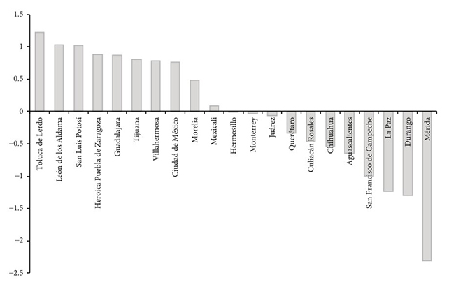
Notes: the index is the average of standardized (z-score) insecurity indicators over the period 2016Q1-2025Q2. Positive values indicate above-average insecurity, whereas negative values indicate below-average insecurity. Cities like Culiacan that have recently experienced a surge in violence may appear relatively less insecure in the ranking, given that the escalation of violence intensified toward the end of the sample period. Source: author’s estimations based on data from INEGI-ENSU.
Figure 1 Overall standardized insecurity index across cities, 2016Q1-2025Q2 (Descending order)
The evidence in Table 5 is based on estimating the model for alternative city subsamples. Broadly speaking, the emerging pattern indicates that, as we exclude the most insecure cities, the negative impact of the three public insecurity measures on housing prices becomes stronger. This is especially true for crime exposure, whose coefficient increases in absolute value when the top six and then the top eight most insecure cities are excluded. Moreover, its statistical significance strengthens from the 5% to the 1% level. By contrast, when the least insecure cities are excluded, the negative impact of the three insecurity measures loses all statistical significance. This is consistent with the idea that the remaining sample is dominated by the most insecure cities, where risk saturation or a violence-normalization effect may prevail.
Table 5 Fixed-effects dynamic panel data models for city subsamples
| Dependent variable: ΔlnP
it
Method: Panel EGLS (Cross-section SUR) Sample (adjusted): 2016Q3-2025Q2 Periods included: 36 Linear estimation after one-step weighting matrix Period weights (PCSE) standard errors & covariance (d.f. corrected) | |||
| Insecurity regressor | |||
| Sample restriction | Model 1: crime expectations |
Model 2: crime perception |
Model 3: crime exposure |
| Full sample: N = 21 | −1.93e-05*** | −2.32e-05*** | -2.62e-05** |
| Excluding the top 6 most insecure cities (N = 15) |
-2.23e-05** | -3.56e-05*** | -5.62e-05*** |
| Excluding the top 8 most insecure cities (N = 13) |
-2.96e-05** | -4.63e-05*** | -8.87e-05*** |
| Excluding the 5 least insecure cities (N = 16) |
-1.43e-06 | 4.53e-07 | -7.08e-06 |
| Dynamic regressor | ΔlnP it-1 | ||
| Control variables | ΔlnCC it , lnY it , lnINFRA it and R it | ||
| Additional controls | Cross-section fixed effects, pandemic dummy, and seasonal dummy variables |
||
Notes: each column reports a separate fixed-effects dynamic panel regression. In addition to the lagged dependent variable, all models include the full set of control variables depicted in equation [1]: construction costs, real mortgage interest rate, public infrastructure, and income, as well as seasonal and pandemic dummies. Asterisks *, ** and *** indicate statistical significance at the 10, 5 and 1% significance levels, respectively. ∆ = first difference operator, ln = natural logarithm. No logarithmic transformation is applied to public insecurity measures or to the real mortgage interest rate, as these variables are expressed in percentage terms.
Source: author’s estimations based on data obtained from the data sources listed in Appendix 1.
As stated earlier, as the most insecure cities are excluded from the sample, crime exposure becomes increasingly influential relative to the other two measures of insecurity. In other words, the hierarchy of effects becomes clearer: housing prices become more responsive to direct experiences of crime and antisocial behavior than to general perceptions or expectations of insecurity. Moreover, expectations that crime-related activity will remain equally bad or worsen consistently constitute the least influential measure, whereas crime perception occupies an intermediate position.
For the sake of brevity, the estimated coefficients of the remaining regressors are not reported in Table 5, since the analysis involves four samples and three measures of insecurity, yielding a total of 12 panel data models. However, broadly speaking, the results are consistent with those reported in Table 4, which corresponds to the baseline model. The coefficient of the lagged dependent variable remains robust and highly stable across the public insecurity measures and city samples. The coefficient of income also remains positive and statistically significant in all 12 regressions. The real mortgage interest rate also maintains a negative and statistically significant coefficient in all but one regression. In this particular case, its p-value is 0.1008, meaning that it is only marginally above the 10% significance threshold. However, broadly speaking, housing price persistence and the core demand-side effects represented by income and the real mortgage interest rate remain robust.
Public infrastructure provision, included mainly as a demand-side variable -an external amenity variable- maintains the expected positive sign across specifications and city samples, although it is statistically significant in only six out of 12 regressions.
Construction costs are regarded as a key supply-side variable. The corresponding estimated coefficient maintains a positive sign and is statistically significant in 11 of the 12 regressions, at the 1% level in nine of them. The estimated coefficient of the pandemic dummy variable maintains a positive sign in all 12 regressions and is statistically significant in ten of them. Finally, the seasonal dummy variables and their reference point, captured by the intercept, are statistically significant in almost 90% of cases (including the intercept in the counting) and display stable signs, reflecting recurrent seasonal patterns in housing price dynamics.
5. Conclusions and policy implications
Broadly speaking, the evidence obtained from the estimation of 12 dynamic fixed-effects panel data models is consistent with the hypothesis that housing prices are more responsive to manifestations of insecurity that can be seen or heard in everyday life -such as street alcohol consumption, robberies, vandalism, drug-related activities, gang presence, and frequent gunshots- than to insecurity that is merely perceived or expected. Although all three measures of insecurity are negatively associated with housing prices, the magnitude and statistical significance of the estimated coefficients across different city samples suggest that the negative effect of crime exposure is the strongest, followed by perceived insecurity and expectations that the crime situation will remain equally bad or worsen.
Perhaps more importantly, Table 5 suggests that, as the most insecure cities are excluded from the sample using an overall standardized insecurity measure, the negative influence of the three public-insecurity indicators becomes stronger, particularly in the case of crime exposure. Put differently, the pattern becomes more pronounced: housing prices appear to respond more strongly to exposure to crime and antisocial behavior than to general perceptions or expectations of insecurity. At the same time, excluding the most insecure cities leaves a sample composed of relatively safer urban areas, where housing prices appear to be more sensitive to public insecurity. By contrast, when the least insecure cities are excluded, so that the remaining sample is dominated by the most insecure urban areas, the negative impact of the three insecurity measures is no longer statistically significant. As discussed earlier, this evidence is consistent with a possible violence-normalization effect, according to which the marginal effect of insecurity on housing prices diminishes as the level of insecurity rises.
These findings are policy-relevant for the following reasons. First, public insecurity may lower housing prices not only through perceived insecurity or expectations that the crime situation will remain equally bad or worsen, but also through visible or audible manifestations of crime and antisocial behavior in everyday urban life. Consequently, policies aimed at protecting housing values -given their close relationship with household wealth and residential investment- should go beyond reducing major crimes and tackle the broader range of antisocial and criminal behaviors captured by crime exposure: alcohol consumption in the streets, robberies and assaults, vandalism, drug dealing or consumption, violent gangs, and frequent gunshots.
Second, the evidence suggesting a decreasing marginal effect of insecurity in the most insecure cities, perhaps due to a violence-normalization effect, does not mean that insecurity has become less harmful to housing markets. Rather, it may indicate that high insecurity levels have already been discounted by market participants and translated into lower property values. In this context, improvements in security conditions should be sustained over time to reverse this damage, since housing prices may not recover immediately due to urban reputation effects, housing-price persistence, and credibility lags. Finally, given that a reduction in visible and audible manifestations of crime and antisocial behavior can help protect household wealth in the long term, encourage residential investment, and lessen disparities between relatively safe and unsafe cities, urban and security policies should be closely coordinated.
As for the other regressors, by and large, our estimations capture housing-price persistence through the lagged dependent variable and unobserved heterogeneity across cities through the fixed-effects specification. This persistence in housing prices shapes the influence of the other regressors, including the pandemic and seasonal dummy variables. On the demand side, the positive and statistically significant income coefficient in the 12 regressions indicates that housing price growth is closely linked to economic activity and earnings. The positive coefficient of public infrastructure provision, which is statistically significant in 50% of the cases, suggests that cities with better water, irrigation, and sanitation systems, reliable electricity and telecommunication services, and improved transportation and urbanization are more attractive to homebuyers, thereby increasing housing demand and prices. Lastly, the negative coefficient of the real mortgage interest rate, which is statistically significant in all but one case, highlights the classical inverse relationship between the cost of mortgage credit and housing demand.
On the supply side, the key variable is construction costs, whose coefficient signals supply-side pressures because it is positive and statistically significant in almost all regressions. Therefore, the costs of construction materials, machinery rental, and labor in the construction industry play an important role in shaping housing prices. In this regard, housing affordability can be enhanced through policies aimed at improving the availability of construction inputs, reducing supply-side constraints, and promoting training programs to raise labor productivity in the sector. Higher labor productivity can reduce unit labor costs in the construction industry and improve housing quality, especially for low- and middle-income families.

