


 nueva página del texto (beta)
 Inglés (pdf)
 Artículo en XML
 Referencias del artículo
 Enviar artículo por email
 Citado por SciELO
  Similares en
SciELO
Similares en
SciELO 
 Permalink
1. Introduction
Recent contributions to the heterodox literature on floating nominal exchange rates have established two important points. The first is that there is really no ‘fundamental’ or equilibrium level of the nominal exchange rate toward which it tends, being ultimately an institutional or policy variable. Vernengo (2001) suggested that more or less sustainable levels of the exchange rate are of a ‘conventional’ nature and much influenced by policy choices, in contrast with the ‘natural’ equilibrium exchange rate determined by the Purchasing Power Parity (PPP) condition. Given this, the second point is that expected exchange rates are always an important determinant of both the spot and forward exchange rates. Harvey (2009, 2019) developed a Post Keynesian portfolio approach to exchange rate determination. His approach strongly emphasizes “FX market psychology”, and that exchange rate expectations are open to multiple determinants, depending on agents’ mental models.
This paper aims to contribute to a third related line of research concerning the implications of different assumptions on the formation of exchange rate expectations. Lavoie and Daigle (2011) have shown the consequences for exchange rate dynamics of the predominance of either ‘chartist’ or ‘conventionalist’ behavior in the FX market. Our purpose here is to introduce elastic exchange rate expectations in the sense of Hicks (1946, pp. 270-272), by assuming that agents always revise their expectations to a certain extent in light of what has actually happened. We do this by means of a simple theoretical framework for the short run2 dynamics of nominal exchange rates under exogenous interest rates and free but imperfect international capital markets, extending the critique of the Mundell-Fleming model in Serrano and Summa (2015), by assuming that agents follow a simple rule of adaptive expectations. We show this is sufficient to demonstrate that elastic expectations lead to changes in the exchange rate, and that these tend to be cumulative.
We also derive some implications for monetary policy and exchange market interventions of this intrinsic instability. We think that our results may be useful both to account for certain alleged ‘puzzles’ found in the literature on the ‘Unconvered Interest Parity (UIP) failure’ and also help to explain the empirical predominance of dirty floating regimes (Calvo and Reinhart, 2002; Frankel, 2019).
After this introduction, our general equation for nominal exchange rate determination in the foreign exchange market is presented in section 2. In section 3, we use it to derive and briefly criticize both the Real and the Uncovered Interest Parity conditions. Following this, in section 4 we introduce elastic exchange rate expectations and derive the associated alternative exchange rate dynamics under adaptive expectations. We then introduce a dirty floating exchange rate regime and derive some implications for monetary policy (in section 5). In section 6, we briefly discuss possible longer run aspects of our analysis. The relation between our simple model results and the empirical literature on the UIP ‘failure’ is then presented in section 7. Section 8 concludes the paper with brief final remarks.
2. A simple framework for the foreign exchange market
2.1. The spot FX market
The balance of payments BPt consists of the current account CAt , the total private capital flows Ft and the change in official reserves ΔRt as shown in equation [1] 3. The balance of payments represented in equation [1] always equals zero4. We also omit pure accounting transactions that do not involve the actual exchange of currencies, and therefore have no impact on the exchange rate. Both to simplify the analysis and because we are concerned only with the very short run, we take the current account balance as exogenously given. The change in official reserves here refers to desired changes. The Central Bank may reduce or increase the quantity of foreign currency available in the spot market. In a “free” or ‘clean’ floating exchange rate regime, the change in reserves is zero.
In equation [2], we split the private capital flows into the long run foreign capital flows FLRt, and the short run capital flows FSRt, the latter defined as all those that depend on interest-rate differential5. FLRt is considered exogenous throughout the paper. In equation [3], the short run capital flows FSRt are determined by the difference between the domestic interest rate it and the reference foreign interest rate i*t. We add up the spread associated with the country-risk ρt and the expected devaluation of the exchange rate6 (Eet+1/Et) to the interest rate differential. The parameter γ represents how much capital flows respond to the interest-rate differential, the country-risk and the expected rate of change of the nominal exchange rate. The changes in agents’ net financial positions, including changes in banks’ holdings of foreign exchange, are included as part of the short run flows in the spot foreign exchange market7.
In equation [4], the spot exchange rate is the endogenous variable that will adjust to balance the demand and supply of foreign exchange.
In equation [5], we express equation [4] in terms of the expected rate of change of the nominal exchange rate, while in equation [6] it is expressed in terms of the level of the nominal exchange rate.
Therefore, the current level of the nominal exchange rate is determined by its expected value, the return differential between foreign and domestic assets, the degree of response of short run capital flows to this differential, the changes in official reserves, the net current account and the long run capital flows balances.
2.2. The forward FX market8
According to Keynes (1923, pp. 94-95) spot and forward markets are tied through arbitrage because of the Covered Interest Parity (CIP) condition. The CIP expresses a non-arbitrage condition according to which the forward premium in the FX forward market must equal the interest differential, otherwise investors would obtain non-risky profits out of this difference. This non-arbitrage condition determines the necessary relation between the forward and spot nominal exchange rates but does not directly determine the levels of any of these two variables. This is shown in equation [7]:
The forward market is the market for exchange to be delivered in the future. Thus, the difference between the spot and the forward nominal exchange rates must be equal to the difference of interest rates in both currencies, reflecting the costs of borrowing in one currency and investing in the other and respecting the ‘no-arbitrage condition’. In other words, this is the same thing as the Covered Interest Parity, which is largely verified in the empirical literature (Sarno, 2005; Lavoie, 2014, chap. 7)9.
It is clear from this perspective that any change in the spot market must be immediately connected10 also to a proportional change in the forward market. Hence, speculation does not occur by some mismatch between forward and spot rates. It occurs because someone wants to buy low to sell at a higher price at the subsequent period (or vice versa), and this depends only on current expectations about the actual exchange rate that will prevail in the future. According to Kindleberger: “(…) the forward contract in foreign exchange introduces no real change into foreign exchange theory (Kindleberger, 1939, p. 179)”.
Using this connection between forward and spot markets, we can easily also derive the equation that determines the level of the nominal forward exchange rate as shown in equation [8].
Therefore, the level of the forward nominal exchange rate is determined by the expected value of the spot exchange rate, the degree of response of short run capital flows to this differential, the changes in official reserves, the net current account and the long run capital flows balances.
We can see in equations [6] and [8] that both the spot and the forward exchange rate are influenced by the expected spot exchange rate. Speculation causes changes in Eet+1 and impacts both markets at the same time. Note that in equation [8], the expected spot exchange rate is not, in general, equal to the forward exchange rate, because of the effect on the spot market of the variables representing the flows of foreign exchange coming through the net current account and capital flows11. Because of the CIP condition, the forward exchange rate is also affected by these flows. The forward exchange rate would be equal to the expected spot exchange rate only under the very unrealistic assumption of perfect and efficient international capital markets in which interest-rate differentials would always bring an infinite amount of capital. This can be seen in equation [8] by setting γ = ∞.
The fact that the forward exchange rate does not directly determine the level of the spot exchange rate does not mean that existence of forward markets has no effect on the determination of the spot exchange rate. According to Kindleberger the real contribution the forward market makes is: “(…) in providing inexpensive opportunities for hedging and speculation or the real character of the forward contract” (Kindleberger, 1939, p. 181).
We can represent this effect of forward markets in the exchange rate dynamics through the parameter γ, which measures the sensitivity of short run foreign investment to the interest-rate differential. The existence of large forward markets would tend to lead to higher levels of γ, both for short run capital inflows at outflows.
2.3. Exchange rate expectations
We argue that exchange rate expectations can be either inelastic or elastic in the sense of Hicks (1946, pp. 270-272). Inelastic expectations are independent of past observations of the exchange rate and could be determined by market conventions, inflation expectations, etc. By contrast, elastic expectations are influenced by past observations of the actual exchange rate. In this paper, we will represent these different assumptions by means of a simple equation of adaptive expectations as shown in equation [9] 12.
If the parameter β equals zero, then expectations are inelastic. If β equals one, then expectations follow the naïve version of adaptive expectations. If β is in the interval between zero and one, then expectations are elastic, but may also be affected by exogenous shocks. In this case, the initially expected level of the exchange rate is exogenous but the point is that this will be revised to a certain extent according to the actually observed values13.
3. Exchange rate determination under inelastic expectations
3.1. The neoclassical approach
In perfect international capital markets, there is free capital mobility and also there are no credit constraints, and an infinite amount of capital is always instantly available at an interest rate slightly above the international rate of reference.
In our model, the assumption of perfect international capital markets is represented by an infinite speed of adjustment of short run capital flows in response to interest-rate differentials (Gandolfo, 2016, p. 60). In equation [5], the parameter γ will be infinite, and the second term on the right-hand will tend to one. It also implies that the sovereign risk ρ equals zero.
Combining the assumptions of perfect capital markets and of inelastic exchange rate expectations β = 0, we can rewrite equation [5] as:
Equation [10] is the traditional equation associated with the UIP condition. Perfect capital markets and inelastic expectations imply that the interest rate differential must coincide with the expected currency devaluation. Considering that the Central Bank exogenously determines the nominal interest rate, and the expected level of the nominal exchange rate is given, equation [10] determines the level of the current spot exchange rate (Blanchard, 2017, chap. 19)14. Therefore, starting from an equilibrium situation, an increase (decrease) of the interest-rate differential causes an initial appreciation (depreciation) of the level of the spot exchange rate. Since the expected level of the exchange rate is not affected, this appreciation (depreciation) of the spot rate creates an expectation of a future depreciation (appreciation), which is in line with the positive interest-rate differential according to the UIP. Hence, despite the shock caused by the change in the domestic interest rate, the level of the expected exchange rate does not change, but the level of the spot exchange rate adjusts to make the expected rate of change of the exchange rate equal to the interest-rate differential.
In the neoclassical approach, because of the assumption of the neutrality of money, in the long run this expected rate of change of the nominal exchange rate is further assumed to be equal to the differential of domestic pt and foreign p*t rates of inflation. These assumptions guarantee both the PPP and Real Interest Parity conditions15.
3.2. The heterodox approach
From a heterodox perspective, there is no assumption of long run neutrality of money and hence no tendency to the PPP condition. In the latter case, however, the fact that changes in the nominal exchange rate have a strong effect on the rates of inflation in many countries may give the impression that PPP tends to prevail in the long run but in fact this is not the case, as the causality runs from the exchange rate to cost-push inflation and not the other way around (Vernengo, 2001).
In this heterodox perspective, even with free mobility of capital, the international capital markets are seen as imperfect and external credit rationing is an important determinant of the balance of payments constraint (Lavoie, 2014, chap. 7; Serrano and Summa, 2015). Therefore, without perfect capital markets, the response of capital flows to interest-rate differentials γ is not infinite (and may well fall to zero as we will see in the next section). In this case, even when the expected nominal exchange rate is assumed to be inelastic and determined by market conventions (Harvey, 2009; Lavoie and Daigle, 2011), there is no convergence to the UIP condition. Hence, the level of the nominal spot exchange rate is given by equation [6].
4. Exchange rate dynamics, elastic expectations and exogenous interest rate under imperfect capital markets
4.1. Imperfect capital markets and elastic exchange rate expectations
In order to present a more realistic alternative model, we first assume free but imperfect capital markets in the sense of Serrano and Summa (2015). In this view, the degree of response of short run capital flows to this differential γ is never infinite. Moreover, this parameter falls to zero in situations in which there is a ‘sudden stop’ or international credit rationing for capital inflows. In this situation, however, γ will remain positive and probably quite high for capital outflows. The nature of the response of short run capital flows to interest-rate differentials will depend on the perception in international markets of the structural situation of the country’s balance of payments. This will be reflected in the country’s sovereign spread ρt, that for each country will depend both on the general conditions of international credit markets and on the specific market assessment of the specific country’s actual risk of default on its foreign currency liabilities. As the actual balance of payments situation of a country worsens, the risk premium tends to increase and beyond a certain point, international credit will be severely rationed.
We must also drop the assumption of inelastic exchange rate expectations because it is too unrealistic to assume that expectations will never be revised to any extent in the light of what actually happened. From now on, we will assume that exchange rate expectations are always to some extent elastic. In terms of our adaptive-expectations equation, this means that β > 0 in equation [9] above.
Elastic expectations have been formalized in terms of ‘chartist’ behavior of some agents, which simply project that the recent past change in actual exchange rates will continue in the future. Our approach differs from that in two aspects. First, we make expectations directly about the level of the exchange rate and not of its change. Second, in our formulation there is room for an initial exogenous level of the expected exchange rate, and it is this initial level that always will be at least partially revised according to what actually happened.
Lavoie and Daigle (2011) model exchange rate expectations assuming heterogenous agents. Some agents are called ‘conventionalists’ and have a conventional and inelastic expectation about a long run level of the nominal exchange rate16, while others follow a ‘chartist’ behavior. In contrast, in our model, agents are neither exclusively ‘conventionalist’ nor ‘chartist’. Whenever they think there is some reason for the past to be very different from the future, they change the initial expected level of the exchange rate exogenously. However, they also will not keep holding those initial expectations unchanged over time if they perceive that they do not correspond to what happened in reality.
As it is well known (Gandolfo, 2005, pp. 29-31), adaptive expectations of this sort (equation [9]), with β greater than zero and smaller than one, starting from any initial exogenous level, always converges to:
The influence of any exogenous initially expected level of the exchange rate will tend over time to vanish as expectations are endogenously revised by actual outcomes.
By replacing equation [13] in [6], we get that the level of the spot exchange rate is given by:
Equation [15] shows that in our model with elastic expectations, there is no equilibrium level of the nominal exchange rate but just a tendency towards a particular rate of change of the exchange rate. This rate of change will be inversely related to the interest-rate differential and to the net current account and long run capital inflows. Moreover, discretionary purchases of reserves by the Central Bank are positively related to the rate of change of the exchange rate.
Of course, at any given time there may be changes in any of the independent variables of equation [15], or in the exogenous initially expected level of the exchange rate that will make the actual rate of change of the exchange rate move away from its previous trend. However, what matters to us is that, after any exogenous shock, the spot exchange rate will be always tending back to the rate of change given by equation [15].
We can illustrate this tendency of the rate of change of the exchange rate by means of simple simulations. We do this by first replacing equation [9] into [6] and then giving values for all the parameters, namely, the initially expected level of the exchange rate and the other independent variables17.
Let’s consider a situation where the interest-rate differential (including risk) is zero, but the long run inflows of capital are assumed not to be large enough to compensate a negative net current account, and the Central Bank does not intervene in the FX market (a free-floating regime). The following condition holds:
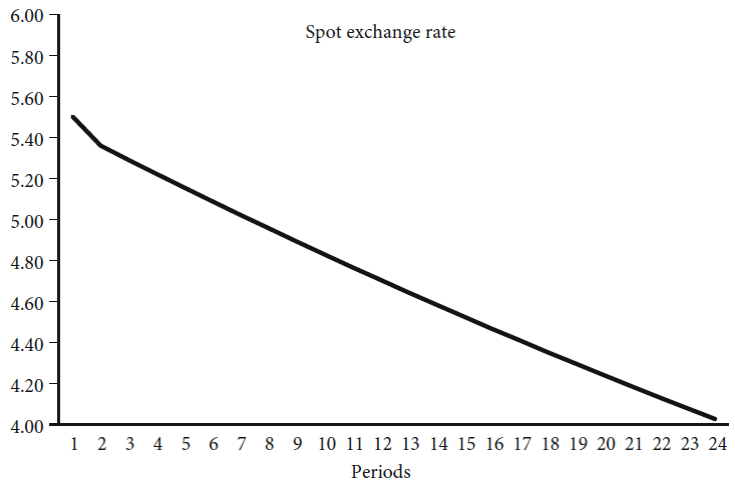
Figure 1 shows us that in this case, the level of the exchange rate tends to continuously depreciate over time at the rate described by equation [15]. Next, we suppose a situation in which the current account deficit is still assumed to be, in absolute terms, larger than the long run capital inflows. However, now we also assume a considerable positive interest-differential (including risk) attracting short run capital flows, such that the following condition holds:
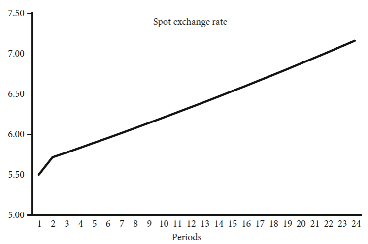
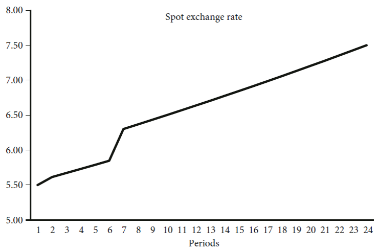
Figure 2 shows a process of continuous appreciation of the exchange rate (again, there is no intervention in FX markets). Finally, we can return to our first simulation and condition [16] to show what happens if an exogenous shock in exchange rate expectations occurs. Suppose that a new, higher initially expected level of the exchange rate appears in period 6 because of an exogenous expectation shock. The result is shown in Figure 3. The shock causes a more rapid increase of the nominal exchange rate from period 7 on. However, the exchange rate returns later to its previous rate of depreciation as given by equation [15].
Source: Authors.
Figure 3 Simulated exchange rate devaluation process (with an exogenous shock on expectations)
Post Keynesian authors (Harvey, 2009) have argued that expectations in FX markets destabilize such markets. As imbalances in the FX markets give rise to changes in exchange rates rather than leading to an equilibrium level of this variable, our results show that in fact it is elastic exchange rate expectations that make free floating exchange rate regimes intrinsically unstable.
The ultimate cause of this basic instability is that, contrary to markets for produced goods, in the FX market there is no supply (or normal) price that would limit the cumulative effects of speculation (Kaldor, 1976). In the case of produced goods, a demand price much greater than the supply price will eventually lead to a large increase in their supply reducing the demand price. And a demand price lower than the supply price will tend to cause a large reduction in their supply causing the demand price to rise. Hence, exchange rate expectations have no objective anchor, apart from the policies and announcements of the Central Banks (when those are credible). In other words, there is no such a thing as a ‘fundamental’ level of the exchange rate, as the spot exchange rate only reflects the Central Bank’s policy choices and the external constraints, both regarding trade and finance of each country (Vernengo, 2001).
5. Dirty floating exchange rate regimes
5.1. Central Banks’ interventions
Although we have shown that free floating regimes are intrinsically unstable, in the real world we do not observe such extreme instability in the FX markets. But this is actually the result of policy interventions of various types as in fact no country really has a completely free floating exchange rate regime, as shown in the ‘fear of floating’ literature (Calvo and Reinhart, 2002; Steiner, 2017; Frankel, 2019)18.
Central banks try to limit the instability associated with free floating regimes by managing the exchange rate using various types of intervention. A frequent instrument used by Central Banks is spot FX market interventions: direct trading of international reserves in spot markets (Patel and Cavallino, 2019). Other intervention tools used are derivatives traded in forwards markets (Farhi, 2017). Also, Central Banks can set the domestic nominal interest rate to affect interest-rate differentials and short run capital flows. Sometimes, instead of changes in the domestic interest rate, Central Banks introduce taxes on short run capital inflows or outflows to affect the interest-rate differentials net of taxes.
5.2. Reserve interventions
One way of intervening in a dirty floating regime is when the Central Bank either announces or just acts to achieve a floor Emin or a ceiling Emax to the exchange rate to control the expected rate of change of the spot exchange rate. Given its target, the Central Bank will buy or sell the necessary quantity of international reserves to reach it.
When there is a strong tendency towards exchange rate appreciation, the Central Bank may set a floor Emin≥Eet+1 to stop this process. In this case, the Central Bank must accumulate reserves until it completely stops the expected appreciation. In that case, it is reasonable to assume that the Central Bank can hit its target since it does it by accumulating reserves paying for them in its own currency. We can show this by modifying equation [6] to include the target floor Emin and solving for the necessary purchase of reserves:
Things become much more complicated when the Central Bank tries to target a ceiling when there is a tendency towards a continuous depreciation. In this case, Emax<Eet+1 and the Central Bank must sell the necessary quantity of international reserves to reach E max as we see in equation [19] below:
However, since international reserves are finite and denominated in a currency that the Central Bank of this country cannot issue, its capacity to hit and maintain the exchange rate target will depend on the availability of potentially scarce international reserves. Moreover, the Central Bank's target may not be credible if the traders in the FX market have reasons to doubt the capacity of the Central Bank to sell enough reserves to stop the process of exchange rate depreciation. Speculative attacks may happen if agents perceive that the monetary authority will not be able to sustain the target, something which can accelerate the process of depleting international reserves.
Note that in our model any purchase or sale of international reserves will affect the level of the spot exchange rate according to equation [6]. However, if this intervention is once for all, this effect will be temporary. Only if the Central Bank is prepared to buy or sell foreign exchange reserves in the amount given by equations [18] or [19] in each period the level of the spot exchange rate can be stabilized over time19.
5.3. Dirty floating and monetary policy
Figure 4 expresses our model in interest-rate-level of the exchange rate plane. According to equation [15], the nominal interest rate ieqt that will stabilize the exchange rate at some level over time will be given by:
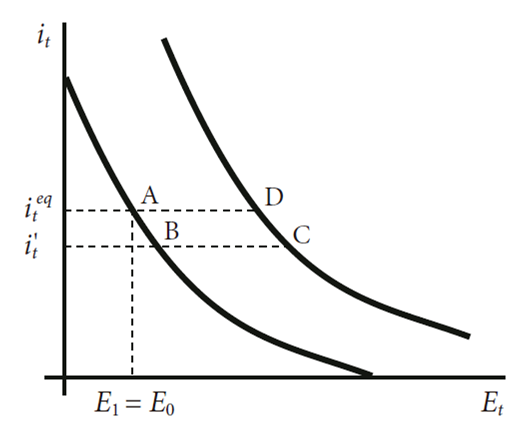
This particular level of the nominal interest rate ieqt is determined by two sets of variables. The first set is defined by the sum of the international rate of reference and the country-risk. The second set corresponds to the desired change in international reserves (corresponding to Central Bank purchases) minus the sum of the current account and the flow of long run capital flows. These variables are divided by the short run capitals’ sensitivity coefficient to the interest differential. If the Central Bank reduces the interest rate to i't, everything else remaining constant, the exchange rate will at first depreciate because the interest-rate differential is smaller, and the economy will move from point A to point B. However, because the expectations are elastic, the depreciation will continue through time, so our initial curve in Figure 4 will shift upwards, and the economy will move from point B to C. This process will continue if the interest rate remains below ieqt.
In order to interrupt this cumulative process of depreciation, the Central Bank has to raise the interest rate back to ieqt. In this case, the depreciation process will stop but the exchange rate will be at a more depreciated level compared to the initial position (point D). But if the Central Bank wants to restore the initial level of the exchange rate E0, it will need to raise the interest rate above ieqt for a while, causing an appreciation and shifting back the curve to the left in Figure 4.
However, if the Central Bank wants to have a specific target for the level of the exchange rate, and at the same does not want to reduce its international reserves below a certain point, then it must set the domestic interest rate at the level that is necessary to generate an interest differential large enough to attract short run international capitals and stop the process of depreciation. The domestic interest rate must be equivalent to:
Equation [21] shows the domestic interest compatible with the targeted level of the exchange rate Etargett rate. The last point to notice is that this kind of policy of setting floors and ceilings can be dynamic in the sense that the Central Bank can change its policy objectives very often (for example, daily). So, in the process of exchange rate appreciation, the Central Bank can at the same time set floors each day and control the pace of exchange rate appreciation. It is entirely possible to the Central Bank by setting its nominal interest rate (and interest differentials) to accumulate reserves and appreciate domestic currency at the same time (as long as international conditions allow it). In other words, this is what has been called ‘systematic managed floating’ regime (Frankel, 2019). Note in managed floating regimes policy tools such as interest rates, taxes, sale and purchases of reserves, forward market interventions and announcements may be used to different extents and in different combinations over time, such that the actual degree of appreciation or depreciation that will be observed in reality will depend both on external shocks and the economic policy objectives.
6. Beyond the short run
The focus of this paper has been on the very short run dynamics of the nominal exchange rate, under the provisional assumption that the balance of current account remains constant during the fast adjustment process of financial capital flows.
However, even in the very short run, in which we can safely take the volume (quantities) of imports and exports as basically given, as the nominal exchange rate is changing all the time, the current account balance in foreign currency could only have been taken as given because we made two implicit special additional assumptions. The first is that the country under consideration is a price taker in all international markets for all goods and (non-factor) services it exports. The second is that all foreign liabilities of this country are effectively denominated and paid in foreign currency. Only under these assumptions both the balance of trade of goods and services and the net income to abroad can remain constant as the nominal exchange rate changes.
But these assumptions, while convenient, are a bit too extreme. It is true that for many developing countries that mostly export commodities, the bulk of their merchandise exports are sold in international markets whose international prices will certainly not change with changes in the nominal exchange rate of one specific exporting country. However, even this type of peripheral country exports a few differentiated products either in a few higher tech niches or typical traditional products of that country whose prices could in principle be seen as basically being set by their costs plus profit margins in domestic currency. Moreover, if we think of non-factor services exports, there are a number of services that are also priced basically in local currency, such as tourism (which is naturally very differentiated between regions). To the extent that the country in question exports such products (goods and services) we would have the traditional, so called ‘initial’, perverse J curve effect (Gandolfo, 2016, chap. 9). A devaluation of the local currency will immediately reduce the inflow of dollar exports.
In terms of our simple model, this effect would tend to accelerate the tendency towards continuous depreciation of the currency in the short run. So, removing the simplifying assumption that the trade balance in goods and services in foreign currency remains constant would only strengthen our results.
Things however could be different when we look at the net income payments to abroad. If we assume the country in question is a net debtor in its own currency, i.e., it does not lend abroad in its own currency (or does very little) but does attract a lot of foreign capital to its domestic assets denominated in its own currency (public debt and stock markets, for instance), then we will have what we could call an ‘inverted financial J curve’ initial effect. In this case an exchange rate depreciation will immediately reduce the foreign currency value of net income payments abroad. And this effect will immediately decrease the foreign currency value of the current account. Therefore, in the case of a tendency towards depreciation, the more a country has effectively borrowed in its own currency the more the tendency towards continuous depreciation may be somewhat dampened. This curious effect seems to have not been widely noticed, but may be of some importance nowadays as the so called ‘original sin’ appears to have been reduced drastically for many ‘emerging market’ countries and many developing countries are now borrowing in their own currency (Akyüz, 2021). Note that we are not talking about the well-known effect that these exchange rate changes have on the stock of foreign net liabilities of the country, but on the current flows of payments arising from those liabilities.
When we try to move beyond the short run and want to consider the possible longer run effects of changes of the exchange rate on the balance of trade of goods and services in our model, we do not have much to add to what is well known in the heterodox literature (Vernengo and Caldentey, 2020). These effects could easily be added to our framework by making export and import volumes being a lagged function of the real exchange rate and of the domestic and foreign levels of economic activity. The lags on the real exchange rate would naturally be much longer than the initial lag on nominal exchange rate expectations in our model. Whether the adjustment of the current account at given levels of local and world activity would counteract the results of our model when there is a tendency towards cumulative depreciation, for instance, would depend on two things. First, on the lasting effect of the nominal exchange rate on the real exchange rate, and second on the well-known Marshall-Lerner conditions, which may or may not hold. But there is also of course the much stronger and certain negative effect of a real devaluation on real wages. This effect reduces domestic consumption and the level of activity, and this reduction leads to a fall in imports, which in reality sadly tends to be the main ‘automatic’ adjusting variable of the balance of payments in many developing countries.
We can then see that beyond the short run many different things may happen in a free-floating regime, some of which may increase even more the intrinsic exchange rate instability. And even in cases when these further effects tend to dampen the instability, these not only may take too long but also, and more importantly, may have a number of undesirable consequences on inflation, income distribution and activity levels. Therefore, we conclude first that considering these longer run effects would reinforce the need for a managed floating exchange rate regime. Moreover, from our analysis, it becomes clear that free floating exchange rate regimes will not automatically eliminate the balance of payments constraint. Hence, the problems related to the longer run external constraint with capital flows need to be addressed with the kind of analyses and policies that come from the structuralist heterodox literature of balance of payments constraint growth (Bhering, Serrano and Freitas, 2019; Thirlwall, 2019).
7. Empirical failure?
As it is well-known, the empirical neoclassical literature on exchange rates have encountered serious difficulties that have been called ‘puzzles’ (Sarno, 2005). One puzzle was found by Meese and Rogoff (1983), who showed that a random-walk model outperforms a structural model (based on the ‘fundamentals’) in forecasting the level of the nominal exchange rate. For us this is not really a puzzle but a result of the fact that there is no long run ‘fundamental’ equilibrium level of the exchange rate. Additionally, the fact that real exchange rates does not present mean reversion is in contradiction with the idea of a long run tendency towards PPP (Sarno, 2005)20.
Another ‘puzzle’ is the so-called ‘UIP failure’. According to the UIP condition, the expected rate of change of the nominal exchange rate should be positively correlated to the interest rate differentials. The empirical estimates usually make use of the ‘Fama regression’ (Fama, 1984), which we represent by equation [22]. In this equation, the expected change of the nominal exchange rate is equal to the forward exchange rate premium plus an error term. Note that the forward exchange rate premium corresponds to the CIP condition. Since a non-arbitrage condition gives this parity, the difference between the forward exchange rate and the spot exchange rate is exactly equal to the interest rate differential. Therefore, the term in parenthesis is equivalent to the interest rate differential and equation [22] is analogous to our equation [10] in which we defined the UIP. Since the expected exchange rate is not an observable variable, one additional step is necessary to arrive at the proper ‘Fama regression’, that is the assumption of the Unbiased Efficiency Hypothesis (UEH). This assumption means that the expected exchange rate is made equal to the actually observed variable in the future (Lavoie, 2014, chap. 7). Equation [22] then becomes equation [23] which is equivalent to the one used for empirical estimations (Fama, 1984; Sarno, 2005; Chin and Frankel, 2020).
For the UIP condition to hold, θ should be equal to one and α equal to zero. However, empirical estimates usually find a negative estimated θ parameter, which is also different from 1 (in absolute value), and a non-zero α. Poor empirical results are so recurrent that there is a specific name in literature for this phenomenon -the ‘UIP failure’. To us, these results far from being a ‘failure’ are fully compatible with our model of exchange rate dynamics (equation [15]). The non-zero α probably represents the fact that with free but imperfect capital markets the interest rate differential is not the only determinant of changes in the exchange rate. This could also be reflected in a θ different from one in absolute terms that may also be capturing the effect of the country-risk21. The negative θ means that exchanges rates tend to appreciate (depreciate) when interest rate differentials are higher (lower), which is opposition to the UIP condition. However, this is precisely the sign that we would expect in our model with elastic exchange rate expectations.
Note that our view is also similar to what Frenkel and Taylor (2006, p. 7) 22 called the ‘speculative’ view of exchange rates. A ‘speculative’ view means that the exchange rate will depreciate when the local interest rate decreases.
The direct consequence of the failure of both the PPP and UIP is the empirical rejection of a long run equilibrium exchange rate defined by the ‘fundamentals’. Exchange rates are volatile, unrelated to differences in prices, and interest rate differentials amplify (rather than mitigate) this volatility. Sarno (2005) calls this the ‘disconnect puzzle’.
The empirical literature about carry-trade also confirms the ‘UIP failure’. The simple fact that carry-trade operations in ‘high-interest currencies’ are often profitable implies that speculation against the UIP can be a profitable strategy (Brunnermeier, Nagel and Pedersen, 2008). On the other hand, this is consistent with our model in which the exchange rate speculation is basically destabilizing, and appreciation or depreciation processes tend to be cumulative23.
8. Final remarks
In this paper we developed a simple theoretical framework to analyze the short run dynamics of nominal exchange rates under exogenous interest rates and free but imperfect international capital markets. In contrast with the neoclassical models based on the UIP condition, we introduced elastic exchange rate expectations and showed that the level exchange rate is intrinsically unstable and do not tend to converge to a long run equilibrium defined either by the neoclassical ‘fundamentals’ or by heterodox ‘conventions’ in a free-floating regime. Note that the form in which we introduced elastic expectations in our model in terms of simple adaptive expectations is in principle consistent but does not require more complex assumptions about heterogenous agents.
Due to this intrinsic instability, Central Banks tend to adopt managed floating exchange rate regimes and intervene using various instruments to prevent cumulative processes and to keep the exchange rate oscillating within certain bounds, according to their general macroeconomic policy targets. In this regime, what frequently appears as pure market ‘conventions’ on expected exchange rates are in fact often reflecting to a certain extent the indications given by the Central Bank actions and announcements of where it wants the nominal exchange rate to go. When these actions and announcements are credible, something that depends on the more structural conditions of the balance of payments situation (including the stock of foreign exchange reserves), they can have a strong effect on market expectations, limiting the intrinsic market instability.

