


 nueva página del texto (beta)
 Inglés (pdf)
 Artículo en XML
 Referencias del artículo
 Enviar artículo por email
 Citado por SciELO
  Similares en
SciELO
Similares en
SciELO 
 Permalink
1. INTRODUCTION
The Observatorio Astronómico Nacional in the Sierra San Pedro Mártir (hereinafter OAN-SPM) is located on the top of Sierra San Pedro Mártir in Baja California, México (2800m, +31° 02” 40’ N, 115° 28” 00’ W). The site excels in sky darkness (Tovmassian et al. 2016; Plauchu-Frayn et al. 2017) and an absence of cloud cover, with approximately 70% and 80% photometric and spectroscopic time, respectively (Tapia et al. 2007). The median seeing measured at zenith at 5000Å varies from 0.55'' to 0.79'', depending upon the study (Echevarría et al. 1998; Echevarría 2003; Bohigas et al. 2008; Skidmore et al. 2009; Sánchez et al. 2012; Ávila et al. 2019) with the most recent measurements favoring a median value near 0.79''. Similar seeing seems to be the rule at nearby sites (Bohigas et al. 2008). Atmospheric extinction is typically 0.13mag airmass−1 in the V band (Schuster & Parrao 2001). Due to these excellent atmospheric conditions and favorable location away from large urban areas, the OAN-SPM is an excellent site for optical and infrared facilities.
In the early 1960’s, a search was begun to find the best site for optical astronomical observations in Mexico (Mendoza 1973). The site was chosen, using, among other information, satellite photographs and on-site testing, as recounted by Mendoza et al. (1972). Subsequent studies during the first years of the observatory’s operation validated the choice of the site (e.g., Walker 1971; Mendoza et al. 1972; Álvarez & Maisterrena 1977). The OAN-SPM was formally inaugurated in 1979.
Tapia (1992) presented a study of ten years (1982-1992) of weather and observing statistics at OAN-SPM site, based upon data reported by the telescope operators. He found that the mean relative humidity was 54% and that the best seasons in terms of cloudlessness and low humidity were spring and autumn. Tapia (2003) and Tapia et al. (2007) updated these results, based upon data spanning 22 years (1982-2002), finding that the fraction of photometric nights was close to 70% for the most recent data and the fraction of spectroscopic nights was approximately 80%.
Michel et al. (2003) presented a four year study with a weather station installed at the 1.5m telescope. They estimated that air temperatures were in the range of −15 to 20°C, the relative humidity showed a seasonal dependence with short variations on short time scales, especially during summer nights. Also, this study reported a range of 733 to 753mb for the atmospheric pressure. Daytime and nighttime wind speeds had median values of 14 and 19km hr−1 with strong winds coming from the SSW direction.
Hiriart (2003) studied the precipitable water vapor above the site over an eight year period (1995- 2002) by measuring the optical depth of the atmosphere at 210GHz, finding a clear peak corresponding to the summer “monsoon” as well as year-to-year variations, e.g., “El Niño” events and the like. Subsequent analysis (Otárola et al. 2009; Otárola et al. 2010) indicated a median precipitable water vapor below 4mm, except in summer.
Here, we continue the tradition of characterizing the site of the OAN-SPM by presenting an analysis of weather variables acquired with the observatory’s weather stations. Since 2006, the OAN-SPM installed weather stations and has operated them continuously as facility instruments. This study describes the data gathered in a consistent and continuous manner by the weather stations during the last thirteen years of operation of the observatory (2007-2019). These stations include sensors for measuring air temperature, atmospheric pressure, relative humidity, wind conditions, water precipitation, solar radiation, evapotranspiration, and the UV index. The equipment used to measure weather conditions is described in § 2, we present our results in § 3 and finally, our conclusions are given in § 4.
2. WEATHER DATA ARCHIVE AND ANALYSIS
The data were acquired with two sets of instrumentation. From mid-2006 to mid-2013, a Davis Instruments weather station (hereinafter DI; Colorado & Hiriart 2007) model Vantage Pro2 Plus was used. From mid-2013, a Vaisala Weather Transmitter (hereinafter VWT) model WXT520 with a Vaisala WINDCAP sensor was installed at OANSPM. The DI weather station has a mechanical cup anemometer (instant readings: 2.5-3 secs.), while the Vaisala WINDCAP sensor of the VWT weather station is ultrasonic (instant readings: 0.25 secs.). The weather data recorded by these stations is currently available from the OAN-SPM homepage3. The basic data that we consider in this paper are air temperature, relative humidity, precipitation, atmospheric pressure, and wind speed and direction. All meteorological variables are monitored continuously. Every five minutes the mean value of the air temperature, relative humidity and atmospheric pressure and the total accumulated precipitation are recorded on the hard disk of the control computer. For the sustained wind speed, the mean value of all instant readings within a five minute interval is determined, while for the gust wind speed, the maximum value in this interval is determined. A systematic error of ±5° degrees is estimated in the alignment process of the station with respect to the true North pole. In Table 1 we present the parameter accuracies for each station as indicated by the manufacturer.
TABLE 1 WEATHER STATION PARAMETER ACCURACY
| Parameter | DI | VWT |
|---|---|---|
| Wind speed | ±5% (< 241km hr−1) | ±3% (< 136km hr−1) |
| Wind direction | ±7° | ±3° |
| Temperature | ±0.5°C (< 43°C) | ±0.2 − 0.3°C (-20 to 20°C) |
| Humidity | ±3% (0 to 90%) | ±3% (0 to 90%) |
| ±4% (> 90%) | ±5% (> 90%) | |
| Pressure | ±0.3mb | ±0.5mb (0 to 30°C) |
| Precipitation | ±4% | ±5% |
The two weather stations are quite similar, with the main difference being a better precision in the wind speed and direction for the VWT station. These two stations have been located at three different sites within the OAN-SPM. The DI station was located on a 6m mast erected upon a rock outcrop about 3m high between the 1.5m and 0.84m telescopes (site 1). The VWT station was first installed on a 6m mast near the Cabaña Azul from August 2013 to November 2015 (site 2), and subsequently on a 6m mast to the west of the 1.5m telescope (site 3). These three different locations are shown in Figure 1.
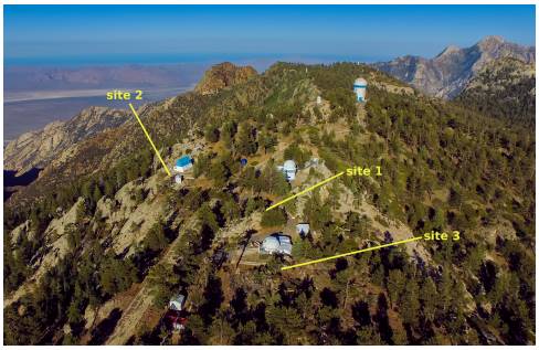
Fig. 1 This aerial view of the OAN-SPM indicates the locations of the DI (site 1) and VWT (site 2 and later site 3) weather stations during period 2006-2019. The photo is courtesy of Eduardo López Ángeles. The color figure can be viewed online.
For this study, we retain thirteen whole years of data (2007-2019), representing ≈97% of the time span available (≈1.3 million 5-minute data points). Table 2 presents a summary of the data. The principal gaps in the data are as follows. There are gaps of approximately two weeks in December 2007 and December 2008, corresponding to the staff holiday period, and there is a gap of several weeks in January 2010, when the observatory was evacuated due to a severe snow storm. During these periods, the weather station was switched off. In addition, there were periods when some of the individual sensors were not functioning, as noted in Table 2.
TABLE 2 WEATHER DATA ARCHIVE
| Year | N of days | % of the year | Location | Comments |
|---|---|---|---|---|
| 2007 | 319 | 87.4% | site 1 | The barometer calibration was incorrect. |
| 2008 | 344 | 94.0% | site 1 | - |
| 2009 | 365 | 100% | site 1 | - |
| 2010 | 351 | 96.2% | site 1 | - |
| 2011 | 365 | 100% | site 1 | The pluviometer was not working. |
| 2012 | 366 | 100% | site 1 | Only 67% of wind data. The anemometer was broken. |
| 2013 | 350 | 95.9% | site 1 & 2 | The wind direction is not reliable for site 2. |
| 2014 | 364 | 99.7% | site 2 | The wind direction is not reliable for site 2. |
| 2015 | 352 | 96.4% | site 2 & 3 | The wind direction is not reliable for site 2. |
| 2016 | 363 | 99.2% | site 3 | - |
| 2017 | 351 | 96.2% | site 3 | - |
| 2018 | 363 | 99.4% | site 3 | - |
| 2019 | 361 | 98.9% | site 3 | - |
Also, the data available concerning the precipitation during winter should be considered a lower limit. The pluviometers for both weather stations are unreliable at sub-zero temperatures (they freeze) and under-record the precipitation that falls as snow. We shall address this limitation in § 3.4.
As a first step in our study, we compare each of the weather parameters collected by the weather stations at the three sites. The distributions of air temperature and relative humidity for both weather stations are similar with no shift between them. On the other hand, for the distribution of the atmospheric pressure, we find a shift of ≈1mb in the distribution of the VWT station compared to the DI station. In addition, when we compare the distributions of the accumulated precipitation of two stations, we find similar distributions, with the VWT distribution slightly shifted to larger values compared to the DI distribution. Because these two weather stations never run simultaneously, we cannot rule out that the differences found are due to an increase of these variables over time. When we compare the distributions for the wind conditions, we find that the only difference among sites was for the wind direction, which lead us to not use the wind direction data collected at site 2, a topic we shall address further in § 3.5.
For the analysis of the data and presentation of the results, we have constructed two data sets: one for daytime and one for nighttime. The nighttime data set includes only data collected when the Sun was ≥ 6° below the horizon (i.e., the period between two consecutive civil twilights) while the daytime data set consists of the data collected during the rest of the day. Both data sets, originally gathered in 5 minute intervals, have been reduced to hourly, daily, monthly, seasonal and annual means, medians, modes or sums depending upon the weather parameter or the issue to be studied. Finally, we define the seasons as follows: winter includes January, February, and March; spring, April, May, and June; summer, July, August, and September, and autumn, October, November, and December.
3. RESULTS
3.1. Air Temperature
The daily maximum and minimum values of the air temperature from 2007 to 2019 are plotted in Figure 2. The air temperature spans the range from −17°C to 23°C over the course of the entire study period. From Figure 2, it can be seen that the daytime temperatures cover a wider range than the temperatures at night. Also, there is a larger dispersion in the temperature during the winter (the valleys in the curves).
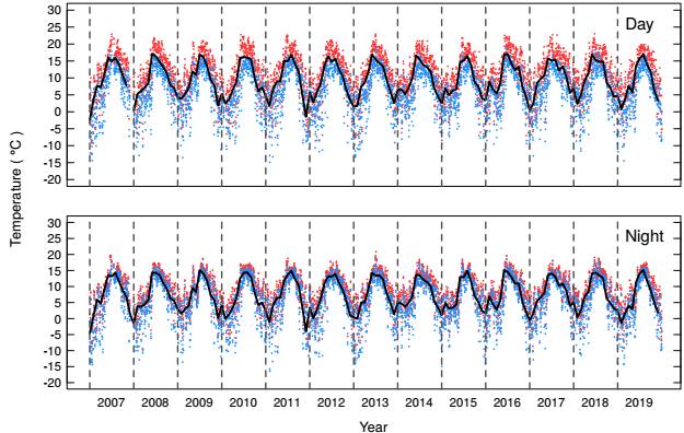
Fig. 2 We present the daily maximum (red) and minimum (blue) air temperature for daytime and nighttime data for the thirteen year time span of our data (2007- 2019). In each panel the black line represents the median monthly air temperature, while the vertical dashed lines indicate the first day of each year. The color figure can be viewed online.
The cumulative distribution of daytime and nighttime air temperatures based upon 5 minute averages is shown in Figure 3a. The median daytime and nighttime air temperatures are 10.3°C and 7.0°C, respectively. From Figure 3a, it can be seen that 90% of the time the air temperature is below 17°C, both day and night. The minimum temperature registered is −16.7°C, with temperatures below 0°C and −4°C occuring only 11% and 4% of the time, respectively. In Figure 3b, we present the cumulative distribution of air temperatures by season for daytime and nighttime. From Figure 3b, it can be seen that the warmest season is summer with a median value of the air temperature of 15.1°C and 13.2°C, for daytime and nighttime, respectively. The coldest season is winter with median values of 4.7°C and 2.7°C, for daytime and nighttime, respectively. Spring is the season with the largest difference between daytime and nighttime temperatures, with median values of the air temperature 11.1°C and 7.9°C, respectively. In autumn, median values of the air temperature are 8.0°C for daytime and 6.0°C, for nighttime.
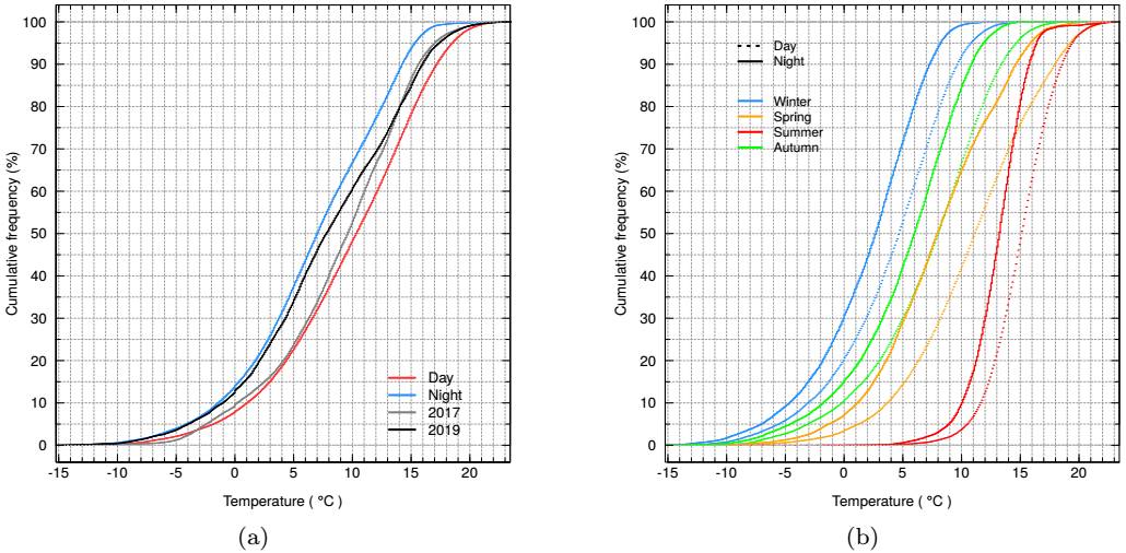
Fig. 3 We present (a) the cumulative distribution of the daytime and nighttime air temperature obtained in the period 2007-2019, based upon the 5 minute averages. The blue line stands for nighttime data, the red line for daytime data, the gray line for 2017 (warmest year, day+night) data, and the black line for 2019 data (coldest, day+night). In (b) we present the cumulative distribution of air temperature by season in the same period for daytime (dotted line) and nighttime (solid line). The blue line stands for winter, the orange line for spring, the red line for summer and the green line for autumn. In both plots, the x-axis does not cover the extremes of total temperature range (-17 to 23°C). Values below -10°C and above 20°C represent only 0.4% and 1.0% of the data, respectively. The color figure can be viewedonline.
We present the monthly means of the air temperature for daytime and nighttime in Table 3 and later in Figure 24 and for each year, the monthly medians are presented in Table 4. The mean temperature at the OAN-SPM has a very clear seasonal variation as can also be seen in Figure 3b. The warmest months are June, July and August and the coldest are December, January and February. The variation between the warmest and coldest months is 13°C (see Table 3). The dispersion about the mean temperatures in Table 3 confirms the impression from Figure 2 that there is more dispersion in temperature in winter and during the day. In Figure 4, we compare the monthly mean of the air temperatures obtained here with those from Álvarez & Maisterrena (1977), Álvarez et al. (2007), and Bohigas & Núñez (2010). All of the data sets are quite similar, except for one point in the 1969-1974 data set, due to a very cold March in 1973 (−3.1°C; see Table 1 from Álvarez et al. 2007).
TABLE 3 MONTHLY MEAN AIR TEMPERATURE
| Month | Day | Night | Day + Night |
|---|---|---|---|
| (°C) | |||
| January | 2.9 ± 4.7 | 1.3 ± 4.4 | 2.1 ± 4.5 |
| February | 3.0 ± 5.0 | 1.1 ± 4.8 | 2.1 ± 4.9 |
| March | 5.1 ± 4.1 | 3.0 ± 3.9 | 4.2 ± 4.0 |
| April | 6.9 ± 4.1 | 4.4 ± 3.8 | 6.0 ± 3.9 |
| May | 9.4 ± 4.2 | 6.8 ± 4.1 | 8.5 ± 4.1 |
| June | 15.4 ± 2.9 | 12.8 ± 3.0 | 14.5 ± 2.9 |
| July | 15.7 ± 1.8 | 13.9 ± 1.7 | 15.1 ± 1.7 |
| August | 15.5 ± 1.8 | 13.8 ± 1.6 | 14.8 ± 1.7 |
| September | 13.3 ± 2.3 | 11.3 ± 2.1 | 12.5 ± 2.2 |
| October | 10.4 ± 3.3 | 8.3 ± 3.2 | 9.4 ± 3.2 |
| November | 6.5 ± 4.2 | 5.0 ± 3.8 | 5.9 ± 4.0 |
| December | 3.3 ± 5.1 | 1.8 ± 4.7 | 2.5 ± 4.9 |
TABLE 4 MONTHLY MEDIANS OF AIR TEMPERATURE
| Month | 2007 | 2008 | 2009 | 2010 | 2011 | 2012 2013 | 2014 | 2015 | 2016 | 2017 | 2018 | 2019 | |
|---|---|---|---|---|---|---|---|---|---|---|---|---|---|
| (°C) | |||||||||||||
| Jan | −3.4 | −0.9b | 3.6 | 4.2d | 3.4 | 4.2 | 0.9 | 5.5 | 1.4 | 2.5 | 0.1 | 6.1 | 3.3 |
| Feb | 1.9 | 4.8 | 2.6 | 1.1 | 0.7 | 1.8 | 1.0 | 5.9 | 6.0 | 8.1 | 1.9 | 1.4 | −0.1 |
| Mar | 6.7 | 5.2 | 4.2 | 2.7 | 5.9 | 4.7 | 6.2 | 4.3 | 4.3 | 5.6 | 7.1 | 3.4 | 2.6 |
| Apr | 6.1 | 6.0 | 5.9 | 5.3 | 7.8 | 7.6 | 6.9 | 6.3 | 5.2 | 4.4 | 8.7 | 8.4 | 6.1 |
| May | 10.3 | 7.5 | 11.0 | 7.9 | 8.3 | 12.7 | 11.3 | 8.9 | 5.8 | 7.0 | 9.9 | 10.4 | 4.5 |
| Jun | 15.2 | 16.0 | 10.0 | 14.7 | 14.0 | 15.3 | 16.0 | 15.7 | 14.0 | 16.4 | 15.0 | 16.0 | 12.9 |
| Jul | 14.3a | 15.7 | 16.0 | 15.4 | 14.5 | 14.2 | 15.2 | 14.8 | 14.5 | 16.4 | 14.7 | 14.8 | 15.2 |
| Aug | 15.4 | 14.5 | 15.3 | 15.3 | 16.1 | 14.9 | 14.3 | 13.2 | 16.1e | 13.7 | 14.2 | 14.4 | 16.3 |
| Sep | 13.0 | 12.3 | 12.8 | 14.4 | 13.1 | 11.8 | 13.0 | 12.1 | 12.9 | 11.4 | 11.1 | 14.1 | 12.9 |
| Oct | 10.1 | 10.7 | 8.3 | 9.1 | 10.9 | 10.0 | 8.6 | 10.8 | 8.2 | 12.6 | 12.2 | 7.6 | 10.5 |
| Nov | 7.3 | 7.1 | 6.9 | 5.1 | 4.1 | 5.9 | 5.6 | 6.0 | 6.2 | 6.5 | 9.6 | 6.0 | 5.3 |
| Dec | ··· | 6.2c | 0.8 | 6.3 | −3.0 | 2.2 | 1.8 | 3.5 | 2.9 | 3.1 | 4.8 | 3.5 | 2.4 |
| Total | 9.6f | 8.7f | 8.2 | 8.2 | 8.4 | 9.0 | 8.4 | 8.8 | 7.6 | 8.4 | 9.4 | 8.4 | 7.5 |
| Day | 10.6 | 9.6 | 9.3 | 9.3 | 9.7 | 9.9 | 9.3 | 9.9 | 8.5 | 9.5 | 10.7 | 9.3 | 8.4 |
| Night | 8.2 | 7.5 | 6.7 | 7.1 | 7.1 | 7.8 | 7.4 | 8.0 | 6.6 | 7.2 | 8.2 | 7.3 | 6.0 |
aNo data for the 3-17th of the month.
b No data for 10-15th of the month.
cNo data for the 14-28th of the month.
d No data for the 20-30th of the month.
eNo data for 26-31th of the month.
f< 95% of data (see Table 2).
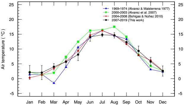
Fig. 4 We compare the monthly mean of the air temperatures from this study with data from Álvarez & Maisterrena (1977), Álvarez et al. (2007) and Bohigas &´ Núñez (2010) and this work. The agreement is generally very good. The color figure can be viewed online.
In the last three rows of Table 4 we report the median annual total (day + night), daytime and nighttime air temperature, which are determined as the median value of the distribution of the daily mean temperatures for each year. By this measure, 2017 was the warmest year in the last thirteen years (see Figure 3a) with daytime and nighttime median air temperatures of 10.7°C and 8.2°C, respectively. The coldest year was 2019 (see Figure 3a) with daytime and nighttime median air temperatures of 8.4°C and 6.0°C respectively. Note that 2007 and 2008 have missing data for the coldest months, so their median temperatures are likely biased to slightly warmer temperatures than the true values.
In Figure 5, we show the cumulative distribution of the daily daytime, nighttime, and day-to-night air temperature variations. We define these temperature variations as the difference between the maximum and minimum temperatures during daytime, nighttime and over a 24 hour day. In a single day, the maximum air temperature variation is smaller than 8°C 90% of the time with a daily median air temperature variation of 5.4°C. During daytime this variation is larger than at night, with median values of 4.8°C and 2.4°C for the day and night, respectively.
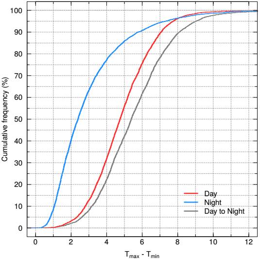
Fig. 5 We present the cumulative distributions of the difference between the maximum and minimum air temperatures during an entire day (gray), during daytime (red), and nighttime (blue). Clearly, the temperature varies substantially less at night than during the day. The color figure can be viewed online.
Figure 6 presents the diurnal variation of the temperature by season. For each season, we determine the mean temperature of the entire day (24 hours) and subtract this temperature from the temperature at a given hour. Values below zero indicate that the temperature is cooler than the daily mean temperature. During daytime (≈06:00 to 12:00 hrs), the air temperature variation is large, typically ∆T ≈ 3°C, with the most extreme variation in the spring, (∆T ≈ 5°C). The air is heated after sunrise with the most rapid phase occurring before 10:00 local time. There is less variation during the middle 4-6 hours of the day. The last four hours before sunset see rapid cooling. From Figure 6, we can se that during the night the air temperature varies little in all seasons.
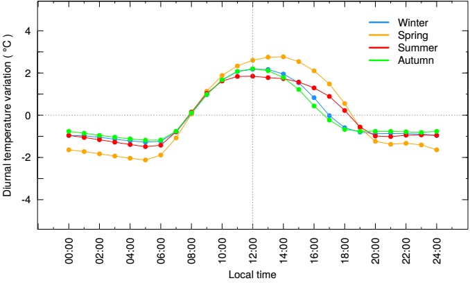
Fig. 6 We present the diurnal air temperature variation by season. To construct these curves, the mean temperature for each entire day (24 hours) is subtracted from the mean temperature for each hour, and the values for the days in a given season are averaged. Again, we see that there is little temperature variation at night. The greatest diurnal temperature variation occurs in spring. The color figure can be viewed online.
In order to estimate how little the air temperature varies during the night, we have estimated the rate of change of the air temperature during nightime. These rates of change are defined as the air temperature at a given hour minus the air temperature an hour before. According to this definition, positive rates indicate heating, while negative rates indicate cooling. In Figure 7a, we present the density functions of the rate of change of the air temperature for 1, 2, 3 hours after the beginning of the night (BoN; Sun is 6° below the horizon, i.e., 24 minutes after sunset) and the period of time between three hours after BoN and three hours before the end of the night (EoN, i.e., 24 minutes before sunrise). We refer to this period simply as “Night” in Figure 7a and 7b. From Figure 7a, it can be seen that after the first hour after the BoN there is a rapid cooling with median value of −0.08°C hr−1. Later, the cooling continues in the second and third hour after the BoN (≈ −0.015°C hr−1), although it is not as rapid as in the first hour after de BoN. In the “Night” period, the cooling has a median value of −0.06°C hr−1. In addition, in Figure 7b, we present the density functions of the air temperature gradients 1, 2, 3 hours before the end of the night (EoN) and the “Night” period previously defined. From Figure 7b, it can be seen that in three hours before the EoN, the cooling is the most rapid with a median value of −0.11°C hr−1. This cooling continues with a median value of −0.09°C hr−1 two hours before the EoN and −0.05°C hr−1 one hour before the EoN. Overall, the air temperature gradually decreases throughout the night at a mean rate of −0.06°C hr−1, with the most rapid cooling one hour after the BoN and the three hours before the EoN.
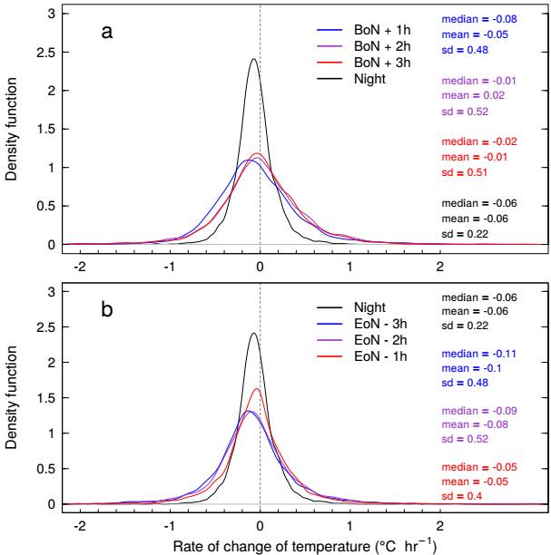
Fig. 7 We present the kernel density plots of the rate of change of the air temperature for: (a) 1h, 2h, 3h after the beginning of the night (BoN) and the period of time including 3 hours after BoN and 3 hours before the end of the night (EoN) or simply “Night” and (b) 1h, 2h, 3h before the end of night and the “Night” period. In each panel, we indicate the median, mean, and standard deviation for each distribution of rates of change with the same color as its respective curve. Negative values of the rates of change of the air temperature gradient indicate cooling, while positive rates indicate heating. The color figure can be viewed online.
In Table 5, we present the dates with the lowest temperatures recorded in the last thirteen years. We have searched for dates where the daytime or nighttime mean temperature was ≤ −10°C. From this table it can be seen the lowest temperatures occur from December to March, usually at night and when the relative humidity is high, perhaps due to the presence of sleet and/or snow. Such conditions are unusual, since the median relative humidity in Table 5 is 70%, which occurs less than 15% of the time (see § 3.2).
Table 6 presents the dates where the daytime mean temperature was ≥ 20°C. As expected, all of these extreme temperatures take/ place in June and July during daytime. When these temperatures occur, the relative humidity is typically below its median value (see § 3.2).
TABLE 5 LOWEST MEAN TEMPERATURES
| Date | Day/Night | Temperature | RH | |
|---|---|---|---|---|
| mean | min | mean | ||
| ( |
(%) | |||
| Jan 13, 2007 | D |
|
|
|
| Jan 13, 2007 | N |
|
|
|
| Jan 15, 2007 | D |
|
|
|
| Jan 18, 2007 | N |
|
|
|
| Jan 19, 2007 | D |
|
|
|
| Jan 19, 2007 | N |
|
|
|
| Jan 22, 2007 | D |
|
|
|
| Jan 22, 2007 | N |
|
|
|
| Mar 16, 2008 | N |
|
|
|
| Feb 2, 2011 | N |
|
|
|
| Feb 3, 2011 | D |
|
|
|
| Feb 3, 2011 | N |
|
|
|
| Mar 18, 2012 | N |
|
|
|
| Jan 11, 2013 | N |
|
|
|
| Jan 12, 2013 | D |
|
|
|
| Jan 12, 2013 | N |
|
|
|
| Jan 14, 2013 | N |
|
|
|
| Dec 31, 2014 | D |
|
|
|
| Dec 26, 2015 | D |
|
|
|
| Dec 26, 2015 | N |
|
|
|
| Dec 29, 2018 | N |
|
|
|
| Jan 1, 2019 | N |
|
|
|
| Feb 18, 2019 | N |
|
|
|
| Feb 22, 2019 | N |
|
|
|
TABLE 6 HIGHEST MEAN TEMPERATURES
| Date | Day/Night | Temperature | RH | |
|---|---|---|---|---|
| mean | max | mean | ||
| (°C) | (%) | |||
| Jul 1, 2007 | D | 20.4 | 22.9 | 18 |
| Jul 2, 2007 | D | 20.5 | 22.2 | 17 |
| Jul 2, 2011 | D | 20.0 | 22.4 | 19 |
| Jun 28, 2013 | D | 20.2 | 22.2 | 31 |
| Jun 29, 2013 | D | 21.2 | 22.5 | 24 |
| Jun 30, 2013 | D | 20.8 | 22.9 | 27 |
| Jun 20, 2015 | D | 20.1 | 21.8 | 10 |
| Jun 19, 2016 | D | 20.9 | 22.1 | 17 |
| Jun 20, 2016 | D | 20.5 | 22.1 | 24 |
| Jul 7, 2017 | D | 20.0 | 22.7 | 35 |
| Jun 22, 2018 | D | 20.5 | 23.1 | 9 |
Studies of global warming (IPCC−SR15 2018 4), performed over long periods of time (≈30 years to correct for short-term natural fluctuations), have shown an increase in the temperature of 0.1-0.3°C per decade. However, this value has been found to be higher in Earth’s land regions than at sea, because oceans lose more heat by evaporation. Also, higher values are measured in the Northern Hemisphere compared to the Southern Hemisphere, because the former has more land surface to absorb more sunlight and more heat. Similarly, there is a seasonal dependence, with higher values for colder seasons. Some Northern Hemisphere mid-latitude winter locations are experiencing a regional warming of more than double the global average.
Álvarez et al. (2007) found an increase in temperature at the OAN-SPM site. They found that temperature increased by 1.3°C from 1969-1974 to 2000-2003 (or 0.4°C per decade). We searched for a trend in temperature as a function of time in our data. The best linear fit to the mean yearly temperature data in the 2009-2019 period does not give a significant variation of the temperature at a 95% confidence level. We present the coefficients of the linear regression fit in Table 7. (We do not include the years 2007 and 2008 since their temperatures are likely biased, as noted earlier.) If we consider data from Álvarez et al. (2007) and perform a linear regression fit to the data for 1969-1974, 2000-2003, and 2009-2019 (a 50 year interval), we obtain an increase in temperature of ≈ 1°C (or 0.2°C per decade see Table 7), but this variation is also not significant at the 95% confidence level.
Additionally, we searched for a change in the number of cold days (daily mean temperature ≤ 0°C) or the number of warm days (mean temperature ≥ 17°C). These two extreme temperatures occur less than 10% of the time. We present these statistics in Table 8. Once again, the linear fits to these data are not statistically significant.
TABLE 7 PARAMETER VARIATIONS (2009-2019)
| Parameter | Coeff.a | Pc | Variation | |
|---|---|---|---|---|
| a±σ | b±σ | (per decade) | ||
| Temperature | 7.94 ± 0.30 (°C) | 0.03 ± 0.04 (°C yr−1) | 0.48 | Not significant |
| Temperatureb | 7.29 ± 0.40 (°C) | 0.02 ± 0.01 (°C yr−1) | 0.06 | Not significant |
| Relative Humidity | 34.71 ± 1.33 (%) | 0.05 ± 0.20 (% yr−1) | 0.82 | Not significant |
| Atmospheric pressure | 728.88 ± 0.27 (mb) | 0.12 ± 0.05 (mb yr−1) | 0.03 | 1.1 ± 0.3mb |
| Precipitation | 124 ± 62 (mm) | 32 ± 9 (mm yr−1) | 0.01 | 286 ± 63mm |
a Coefficients of the linear regression a + bx (x = 1,2,...N years.).
b Using data from 1969-2019 period.
C P value of the slope coefficient of the linear regression.
3.2. Relative Humidity
We present the daily maximum and minimum values of the relative humidity from 2007 to 2019 in Figure 8 for daytime and nighttime data. In this figure, daily maximum and minimum relative humidity values and the monthly median relative humidity for each year are shown. The relative humidity covers a range from 0 to 100% and shows a seasonal variation due to the North American monsoon (Douglas et al. 1993), with summer months being the most humid on average.
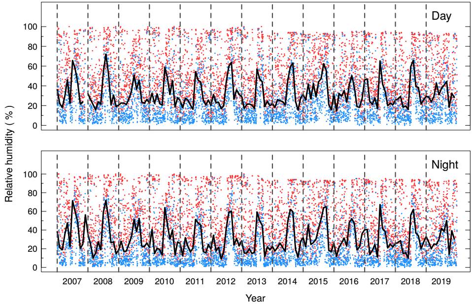
Fig. 8 We present the thirteen year evolution (2007-2019) of the daily maximum (red) and minimum (blue) relative humidity for daytime and nighttime data. In each panel, the black line represents the median monthly relative humidity, while the vertical dashed lines indicate the first day of each year. The monthly median relative humidity peaks in summer due to the North American monsoon. The color figure can be viewed online.
Figure 9a presents the cumulative distribution of the daytime and nighttime relative humidity based upon 5 minute averages. The OAN-SPM is indeed a low humidity site, with a median relative humidity of 30% during the day and 27% at night. Though the distributions are very similar, a Wilcoxon-MannWhitney test confirms that they differ significantly (P value = 8.9 × 10⁻⁹), with the median daytime relative humidity (30%) being slightly greater than the median nighttime value (27%).
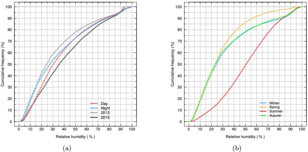
Fig. 9 We present (a) the cumulative distribution of the daytime and nighttime relative humidity obtained in the period 2007-2019, based upon the 5 minute averages. The blue line is for nighttime data, red line is for daytime data, gray line is for 2013 (driest year) data and black line is for 2015 data (most humid year), both data sets include day and nigth data. There is an excess of low humidity values at night compared to during the day. In (b) we present the cumulative distribution by season in the same period. The blue line is for winter, orange line for spring, red line for summer and green line for autumn. The color figure can be viewed online.
The drier conditions at night might seem counterintuitive, but they are mostly due the so called mountain thermal circulation. In their study of the hourly temperature and relative humidity variations at different altitudes at the Kilimanjaro, Duane et al. (2008) found that at low altitudes the relative humidity increases during the night, while at high altitudes this increase is seen during the day (see their Figure 9b). According to these authors, the diurnal variation in humidity it is the outcome of strong upslope moisture transport during the day (via anabatic winds), counterbalanced by downslope transport and drying at night (via katabatic winds). This moisture is produced by the evapotranspiration process of the forest vegetation. At the OAN-SPM site, this effect has also been observed. In their characterization of the Vallecitos site (a valley at an altitude of 2435m and ≈3.5km away from the OAN-SPM site), Tovmassian et al. (2016) found that at Vallecitos site the humidity is much higher at night that in the day, while for the OAN-SPM site it is slightly higher during the day (see their Figure 12). These authors suggest that this might be the result of anabatic and katabatic winds (see their Figure 16). From Figure 9a, it can be seen that 75% of the time, the relative humidity at night is lower than in the day, the rest of the time it is quite similar. The standard requirement for the use of the telescopes is that the relative humidity be ≤85% (and that there be no condensation). At the OAN-SPM, such humid conditions (>85% ) occur during only 6.5% of daytime (300 hours per year) and 7.1% of nighttime (273 hours per year).
In Figure 9b we present the cumulative distribution by season. From this figure, it can be seen that summer is the most humid season with a median value of the relative humidity of 51%, and the driest is spring with a median value of 23%. This is also shown in Table 9, where we present monthly mean values of the relative humidity. April to June (spring) is the driest period at OAN-SPM site while July to September (summer) is the most humid period (see Figure 24).
TABLE 9 MONTHLY MEAN RELATIVE HUMIDITY
| Month | Day | Night |
|
|---|---|---|---|
| (%) | |||
| January |
|
|
|
| February |
|
|
|
| March |
|
|
|
| April |
|
|
|
| May |
|
|
|
| June |
|
|
|
| July |
|
|
|
| August |
|
|
|
| September |
|
|
|
| October |
|
|
|
| November |
|
|
|
| December |
|
|
|
In Table 10, we present the annual median relative humidity for the years 2007 to 2019. Considering day and night data, the driest year was 2013 and the most humid 2015, with relative humidities of 24% and 35%, respectively. This can be seen in Figure 9a, where we show the 2013 and 2015 cumulative distribution of the relative humidity.
TABLE 10 ANNUAL MEDIAN RELATIVE HUMIDITY
| Day | Night |
|
|
|---|---|---|---|
| Year | (%) | ||
| 2007 |
|
|
|
| 2008 |
|
|
|
| 2009 |
|
|
|
| 2010 |
|
|
|
| 2011 |
|
|
|
| 2012 |
|
|
|
| 2013 |
|
|
|
| 2014 |
|
|
|
| 2015 |
|
|
|
| 2016 |
|
|
|
| 2017 |
|
|
|
| 2018 |
|
|
|
| 2019 |
|
|
|
a< 95% of data (see Table 2).
Figure 10 presents the hourly relative humidity and its variation by season. The first panel (a) makes clear that summer is by far the most humid season. There is little difference in the relative humidity between the other seasons. In the second panel (b), for each season, we subtract the mean relative humidity of the day from the relative humidity at a given hour during the day. At a given hour, values below the zero line indicate that the relative humidity is lower than the mean relative humidity of the day.
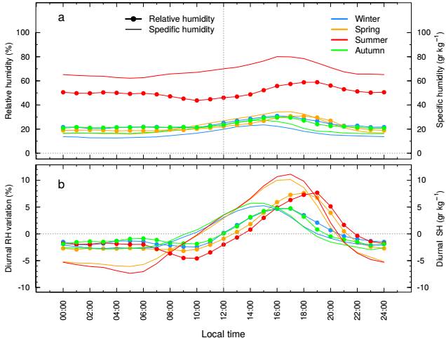
Fig. 10 We present the relative and specific humidity (upper panel) and the diurnal relative and specific humidity variation (bottom panel) by season. Summer is the most humid season (50% relative humidity), with the others all being substantially lower (30% relative humidity). The diurnal variation of the humidity is highest (and similar) in spring and summer while autumn and winter have a smaller diurnal variation. The color figure can be viewed online.
In general, for all seasons, the relative humidity first decreases as the atmosphere warms up during the first hours after sunrise (morning warming), but then increases throughout the rest of the day (via anabatic winds). As the atmosphere cools at sunset, the relative humidity reaches its maximum value, before rapidly falling over the next few hours (via katabatic winds) and reaching a stable value shortly before midnight. Figure 10b indicates that the most extreme (and similar) diurnal variation in relative humidity occurs during the spring and summer seasons.
The relative humidity provides only a partial picture of the water content of the atmosphere at the OAN-SPM. Figure 10 also presents the specific humidity, the amount of water vapor (in grams) present in an air volume of 1 kg, which depends on air temperature, relative humidity and atmospheric pressure. The hourly specific humidity is plotted in absolute value in Figure 10a, while its diurnal variation is plotted in Figure 10b with continuous lines.
Based upon the specific humidity, there is a much greater amount of water vapor in the atmosphere in the summer than in the other seasons (3 times more; Figure 10a). This is not surprising given that both the temperature and the relative humidity are highest in summer, the two factors most affecting the specific humidity. The specific humidity is especially low in winter.
The diurnal variation in summer and spring are quite similar (see Figure 10b), with the only difference being a lower minimum at sunrise (≈05:00 hours) for the summer. In detail, the specific humidity depends upon the relative humidity, the atmospheric pressure and the temperature, but temperature provokes variations of the largest absolute magnitude for the typical conditions at the OAN-SPM. Hence, the diurnal variation of the specific humidity is mostly driven by the diurnal variation of the temperature, though also scaled by the relative humidity. There is a greater diurnal temperature variation in spring than in summer (see Figure 6), but both a lower relative humidity (Table 9) and a smaller amplitude of its diurnal variation. These factors conspire to produce a similar diurnal variations of the specific humidity in spring and summer. As for autumn and winter, their diurnal temperature variations are similar, as are their relative humidities, so they too have similar diurnal variations of the specific humidity.
To investigate whether the relative humidity varies with time, we fit the mean annual values. We find no significant variation as a function of time (see Table 7).
3.3. Atmospheric Pressure
The daily median values of the atmospheric pressure are plotted in Figure 11. Note that we have no data from 2007, when the barometer was not working properly (Table 2). There is a clear seasonal variation of the atmospheric pressure, with high values in summer and lower values in winter. The atmospheric pressure has a median value of 730mb, but varies within the range of 713-737mb (534-552mm-Hg) during the entire period (see Figure 24). As for the air temperature, there is much more variation in the atmospheric pressure in winter than in summer.
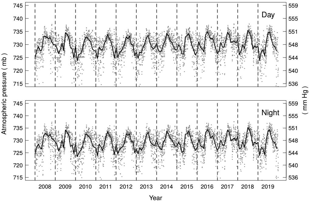
Fig. 11 We present the variation of the daily mean atmospheric pressure for daytime and nighttime data as a function of time (2008-2019). In each panel, the black curve represents the median monthly atmospheric pressure and the vertical dashed lines indicate the first day of each year. There is a clear seasonal variation, with the highest atmospheric pressure in summer and the lowest in winter. There is also a greater variation in the atmospheric pressure in winter.
In Figure 12a, we present the cumulative distribution of the daytime and nighttime atmospheric pressure obtained in the period 2008-2019, based upon the 5 minute averages. The median atmospheric pressure during the day is 730.1mb while at night it is 729.6mb. Although the distributions for the day and night are similar, there is a systematic shift. A Wilcoxon-Mann-Whitney test confirms that both distributions are statistically different (P = 8.4×10⁻¹⁰ that the two distributions arise from the same parent distribution), with the median daytime atmospheric pressure value exceeding the nighttime median value by 0.5mb. As we show later, this difference is mainly due to the thermal atmospheric tides phenomenon.
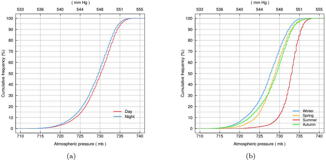
Fig. 12 We present (a) the cumulative distribution of the daytime and nighttime atmospheric pressure obtained in the period 2008-2019, based upon the 5 minute averages. The blue line stands for the nighttime data and the red line for the daytime data. There is a statistically-significant shift between the two distributions, with the daytime values shifted to higher values. In (b) we present the cumulative distribution by season in the same period. The blue line stands for winter, the orange line for spring, the red line for summer and the green line for autumn. The color figure can be viewed online.
In Figure 12b, we present the cumulative distribution of atmospheric pressure by season. From this figure, it can be seen that the season with the highest atmospheric pressure is summer with a median value of 733.1mb. On the other hand, winter has the lowest atmospheric pressure, with a median value fo 727.7mb.
In Table 11, we present the monthly mean values of the atmospheric pressure. The seasonal variation seen in Figure 11 appears in the run of the values. During the summer months (July to September), the atmospheric pressure is the highest (≈ 733mb). This occurs because the OAN-SPM samples the midlayers of the low atmosphere air. In summer, the air at lowest altitudes is heated most and so expands, which raises a greater fraction of the lower atmosphere to greater heights and raises the air pressure at middle heights in the process. The rest of the year, the median atmospheric pressure is below ≈ 730mb (see Figure 12b). As a comparison, at the sea level (e.g. Ensenada, B.C.), the atmospheric pressure ranges between 1002−1025mb and the annual pattern is the inverse, with highest atmospheric pressure during the winter (≈ 1016mb) and the lowest during the summer (≈ 1011mb)5.
TABLE 11 MONTHLY MEDIAN ATMOSPHERIC PRESSURE
| Month | Day | Night | Day + Night |
|---|---|---|---|
| (mb) | |||
| January | 728 | 728 | 728 |
| February | 727 | 727 | 727 |
| March | 728 | 727 | 728 |
| April | 728 | 727 | 728 |
| May | 728 | 727 | 728 |
| June | 731 | 730 | 731 |
| July | 734 | 733 | 734 |
| August | 734 | 733 | 733 |
| September | 732 | 732 | 732 |
| October | 730 | 730 | 730 |
| November | 729 | 729 | 729 |
| December | 728 | 727 | 728 |
Figure 13 presents the variation of the atmospheric pressure throughout the day. Here, we bin the data by season and subtract the daily mean value. The atmospheric pressure varies through two cycles per day whose shape varies seasonally. These variations, also known as thermal atmospheric tides, are complex and not fully understood, but their main cause is the absorption of the solar radiation by the ozone in the stratosphere, aided by water vapor (Siebert 1961; Chapman & Lindzen 1970; Haurwitz & Cowley 1973; Pugh 1987). In the upper atmosphere, the diurnal heating cycle gives rise to diurnal pressure waves, but the dynamic structure of the atmosphere causes the semidiurnal harmonic to be dominant (Pugh 1987; Le Blancq 2011). Hence, we observe two cycles per day.
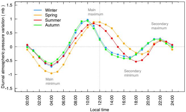
Fig. 13 We present the diurnal and semidiurnal atmospheric pressure variation by season. To construct these curves, we subtract the daily mean value from the hourly means and then average all of the data by season and hour. The diurnal atmospheric pressure variation consists of the main maximum and secondary minimum, while the semidiurnal variation consists of the main minimum and the secondary maximum. The color figure can be viewed online.
The diurnal pressure variation has a minimum and a maximum that occurs at the same time each day in all seasons. In Figure 13, the diurnal minimum (main minimum) occurs at 04:00hrs while the diurnal maximum (secondary maximum) occurs around 22:00hrs. On the other hand, the semidiurnal pressure variation varies seasonally. Its maximum (main maximum) happens earlier in winter and autumn (10:00hrs) compared to spring and summer (12:00hrs) and, likewise, its minimum (secondary minimum) also occurs earlier in winter and autumn (16:00hrs) than in spring and summer (19:00hrs). Overall, the net effect of the atmospheric tides is a lower atmospheric pressure at night compared to the day. The atmospheric pressure variation during the night has a mean value of −0.64, while this value is 0.25 during the day.
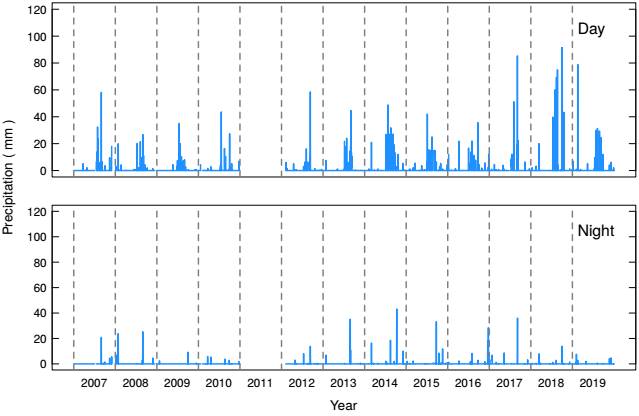
Fig. 14 We present the records (2007-2019) of the daily accumulated precipitation for daytime and nighttime data. The vertical dashed lines indicate the first day of each year. No data were recorded for 2011. These data indicate that there is more precipitation during the day than at night. The color figure can be viewed online.
Studies indicate that the amplitude of atmospheric tides varies with latitude, from about 0.3mb in polar regions to 3.0mb in the tropics (Le Blancq 2011). The amplitude of the tides seen at the OANSPM fits this pattern, since we find an amplitude of ≈ 2mb. Also, there is evidence that the amplitude varies seasonally (Le Blancq 2011). Our results support this finding, since the amplitude is approximately 1.7mb in winter, 1.8mb in spring, and 1.5mb in summer and autumn.
Over the last ten years, the fit to our data shows that the annual mean atmospheric pressure increased by 1.1mb (see Table 7).
3.4. Precipitation
Previous studies of the climate at the OAN-SPM did not include precipitation. These studies relied upon measurements obtained at weather stations in the region of the observatory, at distances up to around 150km (Álvarez et al. 2007) in order to understand the precipitation regime at the top of the mountain. Here, we include rain precipitation data recorded over the last thirteen years. As noted earlier, our data underestimate the precipitation from snowfall since the pluviometers are unreliable in subzero temperatures. Hence, our precipitation data should be treated as a lower limit to the true total precipitation. As mentioned in § 2, we have no data for 2011.
In Figure 14, we show the daily accumulated precipitation for the period 2007 to 2019 for daytime and nighttime data. It is clear that rain is more common during the day than at night. Overall, our records indicate that there is four times more rain during the day than at night.
Two factors affect the precipitation at the OANSPM. On the one hand, the rainy season in the northwest coastal region of Mexico occurs during the winter and it is primarily caused by the southern tails of North Pacific winter storms reaching Southern California and Northern Baja California. On the other hand, in the area surrounding the north end of the Mar de Cortés (Gulf of California), heavy rainstorms occur during the summer, when the precipitation rises to a maximum in August due to the water vapor carried by the North American monsoon (Higgins et al. 1997). Since the Sierra San Pedro Mártir, where the OAN-SPM is located, occupies the highest reaches of the mountain range dividing these two regimes, it is affected by both.
In Table 12, we present the monthly mean accumulated precipitation for daytime and nighttime, which is also plotted in Figure 24. In Table 13, we present the monthly accumulated precipitation for every year. Both Tables 12 and 13, as well as Figure 24, demonstrate that the summer months dominate our precipitation data, though we should keep in mind that we are missing an important fraction of the winter precipitation.
TABLE 12 MONTHLY MEAN ACCUMULATED PRECIPITATION
| Month | Day | Night | Day + Night |
|---|---|---|---|
| (mm) | |||
| January | 6 | 7 | 13 |
| February | 11 | 3 | 14 |
| March | 4 | 2 | 5 |
| April | 3 | 1 | 5 |
| May | 2 | 1 | 2 |
| June | 3 | 0 | 3 |
| July | 76 | 2 | 77 |
| August | 80 | 13 | 92 |
| September | 44 | 10 | 54 |
| October | 20 | 8 | 27 |
| November | 5 | 4 | 9 |
| December | 5 | 8 | 12 |
TABLE 13 MONTHLY ACCUMULATED PRECIPITATION (2007-2019)
| Month | 2007 | 2008 | 2009 | 2010 | 2011 | 2012 | 2013 | 2014 | 2015 | 2016 | 2017 | 2018 | 2019 |
|---|---|---|---|---|---|---|---|---|---|---|---|---|---|
| (mm) | |||||||||||||
| Jan |
|
|
|
|
⋯ |
|
|
|
|
|
|
|
|
| Feb |
|
|
|
|
⋯ |
|
|
|
|
|
|
|
|
| Mar |
|
|
|
|
⋯ |
|
|
|
|
|
|
|
|
| Apr |
|
|
|
|
⋯ |
|
|
|
|
|
|
|
|
| May |
|
|
|
|
⋯ |
|
|
|
|
|
|
|
|
| Jun |
|
|
|
|
⋯ |
|
|
|
|
|
|
|
|
| Jul |
|
|
|
|
⋯ |
|
|
|
|
|
|
|
|
| Aug |
|
|
|
|
⋯ |
|
|
|
|
|
|
|
|
| Sep |
|
|
|
|
⋯ |
|
|
|
|
|
|
|
|
| Oct |
|
|
|
|
⋯ |
|
|
|
|
|
|
|
|
| Nov |
|
|
|
|
⋯ |
|
|
|
|
|
|
|
|
| Dec |
|
|
|
⋯ |
|
|
|
|
|
|
|
|
|
| Total |
|
|
|
|
⋯ |
|
|
|
|
|
|
|
|
| Day |
|
|
|
|
⋯ |
|
|
|
|
|
|
|
|
| Night |
|
|
|
|
⋯ |
|
|
|
|
|
|
|
|
a< 95% of data (see Table 2).
b Pluviometer not working.
In Figure 15, we plot the accumulated precipitation according to the hour of the day for each season. There is no noticeable trend, except for summer. In summer, we find that the heaviest rains occur preferentially between 12:00 to 17:00hrs, which is to be expected since afternoon thunderstorms dominate the precipitation in summer. In other seasons, the precipitation is similar for daytime and nighttime. Since the precipitation in other seasons is determined by larger-scale weather systems, this suggests that the snowfall in winter, largely absent in our data, is similar during the day and night. Hence, we expect the true trend for winter in Figure 15 to be a scaled version of the trend shown.
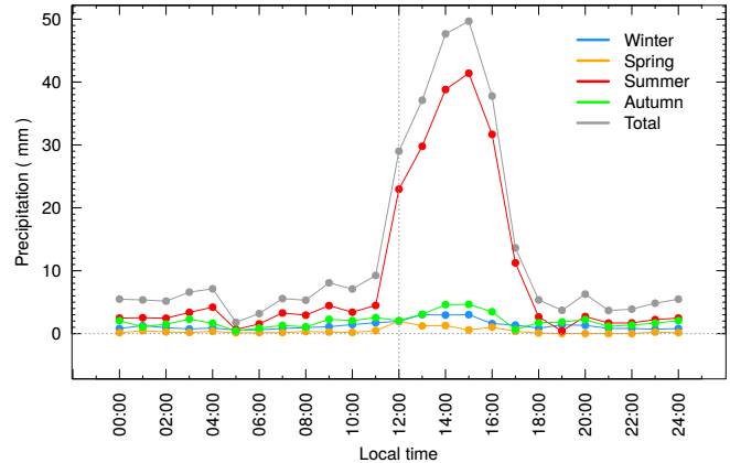
Fig. 15 We present the hourly accumulated precipitation by season as a function of time throughout the day. Except in summer, there is no preferred time for precipitation. In summer, most of the precipitation falls as afternoon thunderstorms. The color figure can be viewed online.
In the last three rows of Table 13, we present the total (day + night), daytime and nighttime accumulated precipitation for 2007-2019. The annual mean rain precipitation at the OAN-SPM is 313±125mm, with ≈ 70% (220mm) falling between July and September. From Table 13, the total is clearly very variable. 2018 had double the annual mean, in part due to abundant rains in October and more than usual during the summer, while 2009 was a year characterized by little precipitation.
Álvarez et al. (2007) reported an annual rain´ precipitation of 449mm using a CONAGUA station (Comision Nacional del Agua) located at the National Park (13km southwest at an altitude of 2080m) during the period 1977-2007, but only 173mm at the OAN-SPM. They reported that 77% of the precipitation at the National Park station occurred during winter time and the rest during spring and summer (see their Figure 2 and Table 3). They also included weather data for a station to the east of the Sierra San Pedro Mártir at a similar latitude as the other two stations. There, precipitation almost only falls in summer, as a result of summer thunderstorms, and the yearly total amounts to 147mm. Therefore, there is clearly a regime change in the precipitation in the vicinity of the OAN-SPM.
At the OAN-SPM, we find at least 50% more rainfall in summer (223mm; Table 12) than reported for the station further east, and double that reported by Álvarez et al. (2007) for the National Park´ weather station. Even if all of the winter precipitation recorded at the National Park station fell at the OAN-SPM, it would amount to only about half the total at the OAN-SPM. If so, the total annual precipitation at the OAN-SPM is likely in the 400-450mm range.
Considering that the rainy days have, on average, a daily accumulated precipitation of 10mm, a heavy precipitation day could be one with ≥ 30 mm. In Table 14 we present the dates with heavy accumulated precipitation in the 2007-2019 period. From this table it can be seen that heavy precipitation days occur always during the summer days and in general are characterized by high temperatures ≥ 10°C, high relative humidity (> 70%) and high atmospheric pressure (≥ 730mb). On the other hand, heavy precipitation days where the relative humidity is low (< 70%) have the highest temperatures > 13°C. However, there were four dates with heavy precipitation, but low temperature (< 9°C) and low atmospheric pressure (< 728mb). These might be the result of cold fronts, which produced the abundant precipitation recorded.
Our findings are undoubtedly biased as a result of our partial winter precipitation records. Clearly, our total annual precipitation must be an underestimate of the true value. Correcting for this would increase the total precipitation in winter. However, given the different nature of the storms, due to weather systems rather than thunderstorms, this winter precipitation is unlikely to be biased to daytime or nighttime. Hence, we expect the true winter precipitation in Figure 15 to be enhanced overall.
TABLE 14 HEAVY PRECIPITATIONa
| Date | Day/Night | Daily | T | RH | Atmosph. |
|---|---|---|---|---|---|
| precip. | mean | mean | pressure | ||
| (mm) | (∘C) | (%) | (mb) | ||
| Jul 29, 2007 | D |
|
|
|
- |
| Aug 31, 2007 | D |
|
|
|
- |
| Jul 15, 2009 | D |
|
|
|
|
| Jul 20, 2010 | D |
|
|
|
|
| Sep 9, 2012 | D |
|
|
|
|
| Aug 26, 2013 | N |
|
|
|
|
| Aug 31, 2013 | D |
|
|
|
|
| Jul 25, 2014 | D |
|
|
|
|
| Aug 17, 2014 | D |
|
|
|
|
| Oct 8, 2014 | N |
|
|
|
|
| Jul 4, 2015 | D |
|
|
|
|
| Sep 21, 2015 | N |
|
|
|
|
| Sep 19, 2016 | D |
|
|
|
|
| Aug 1, 2017 | D |
|
|
|
|
| Sep 2, 2017 | D |
|
|
|
|
| Sep 3, 2017 | N |
|
|
|
|
| Jul 10, 2018 | D |
|
|
|
|
| Jul 29, 2018 | D |
|
|
|
|
| Aug 11, 2018 | D |
|
|
|
|
| Aug 20, 2018 | D |
|
|
|
|
| Oct 1, 2018 | D |
|
|
|
|
| Oct 15, 2018 | D |
|
|
|
|
| Feb 14, 2019 | D |
|
|
|
|
| Ago 6, 2019 | D |
|
|
|
|
a Accumulated precipitation (≥ 30mm).
The yearly totals in Table 13 show a clear increase in precipitation in recent years compared to the years up to 2012. Alternatively, if we fit these data as a linear trend, we find an annual increase in precipitation, on average, of 30mm more precipitation per year for the 2009-2019 period (99% confidence level). The values and uncertainties of the coefficients of the linear fit are shown in Table 7. In Figure 16 we present the linear fit to our data in the 2009-2019 period (blue line). In addition, we have included the linear fit for the 2007-2019 period (2007 and 2008 are years with <95% of data; see Table 2) to verify if this increase in precipitation over the years is also maintained in this period. We find that this trend continues, although it is slightly lower, with 20mm per year (99% confidence level). Álvarez et al. (2007) presented a weather model (see their Figure 7) that predicted that precipitation would increase from 2007, equalling its long-term average around 2015 and increasing to a maximum between 2020 and 2035. Hence, the increase in total annual preci/pitation that we find supports their scenario.
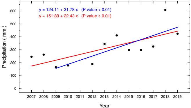
Fig. 16 We present the linear fits to annual precipitation data for the 2009-2019 period (blue line) and 2007-2019 period (red line). Both linear fits have a confidence level of 99%. The color figure can be viewed online.
Studies of global warming have shown that regions with the largest increases in heavy precipitation events include several high-latitude regions, mountainous regions, eastern Asia and eastern North America (IPCC−SR15 2018). We count the number of days per year with measurable daily precipitation (P ≥ 1mm) and the number of days with daily heavy precipitation (P ≥ 10mm) for the 2009-2019 period (only years with ≥95% data) and present this information in Table 15. We do not find any significant variation in the number of days with precipitation or heavy precipitation, but rather a correlation with the total precipitation.
3.5. Wind Speed and Direction
The DI and VWT weather stations deliver two wind speeds: the sustained wind speed and the wind gust speed. For a description of how these two parameters are determined, we refer the reader to § 2.
The DI and VWT stations were installed at different heights in the three sites, so we have normalized all wind speeds (both sustained and gusts) to a common 7 m height using equation (1) of Bohigas & Núñez (2010) (hereinafter referred to as BN10). Their fit to the median value of the wind speed as a function of height, h, is
While equation 1 was derived for another nearby site, a relation of this form is expected generally (e.g., Stull 1988). In Figure 17, we present the cumulative distributions of the sustained wind speed for the three sites before and after applying the normalization from BN10. Clearly, equation 1 is reasonably effective at matching the three wind speed distributions from the three sites, especially since our focus is upon the general conditions at the OAN-SPM. The small residual differences are presumably due to differences in the vertical variation of the wind speed at the three sites relative to that at the site studied by BN10. It is likely that the smaller differences between sites 1 and 3 reflect that these sites, like that studied by BN10, are on the south side of the ridge whereas site 2 is on the north side. Since the strongest winds come predominantly from southerly directions (e.g., Figure 22), site 2 should be somewhat more protected by the local terrain than are sites 1 and 3. This may explain why the wind speed distribution for site 2 has a slightly lower proportion of the highest wind speeds.
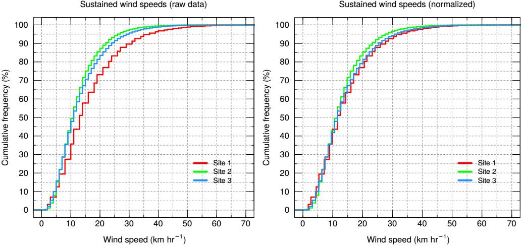
Fig. 17 We present the cumulative distributions of the sustained wind speeds for the three sites before (left panel) and after (right panel) applying the normalization from Bohigas & Núñez (2010). These graphs include data for the period 2007-2019, based upon the 5 minute average values. The color figure can be viewed online.
As noted in § 2, the distribution of wind directions for site 2 seems to be rotated by 45° when compared to sites 1 and 3, probably due to an error in the orientation of the sonic anemometer at site 2. Alternatively, the orography or buildings around site 2 may be to blame. On the other hand, the cumulative distribution for the wind speed does not appear anomalous. Given the discrepancy with its wind directions, we discard the wind direction data gathered at site 2 from this study. But when only the wind speed is needed, we include the data from site 2. When both the wind speed and direction are needed, we discard the data from site 2 because its wind direction parameter it is not reliable.
The daily maximum and minimum values of the sustained wind speed are plotted in Figure 18 for daytime and nighttime. There are gaps in the data for the years 2007, 2008, 2009 and 2010 winters because the DI wind vane froze, and in 2012 the anemometer was broken (see Table 2). From Figure 18, it is also clear that the sustained wind speed is lowest in summer.
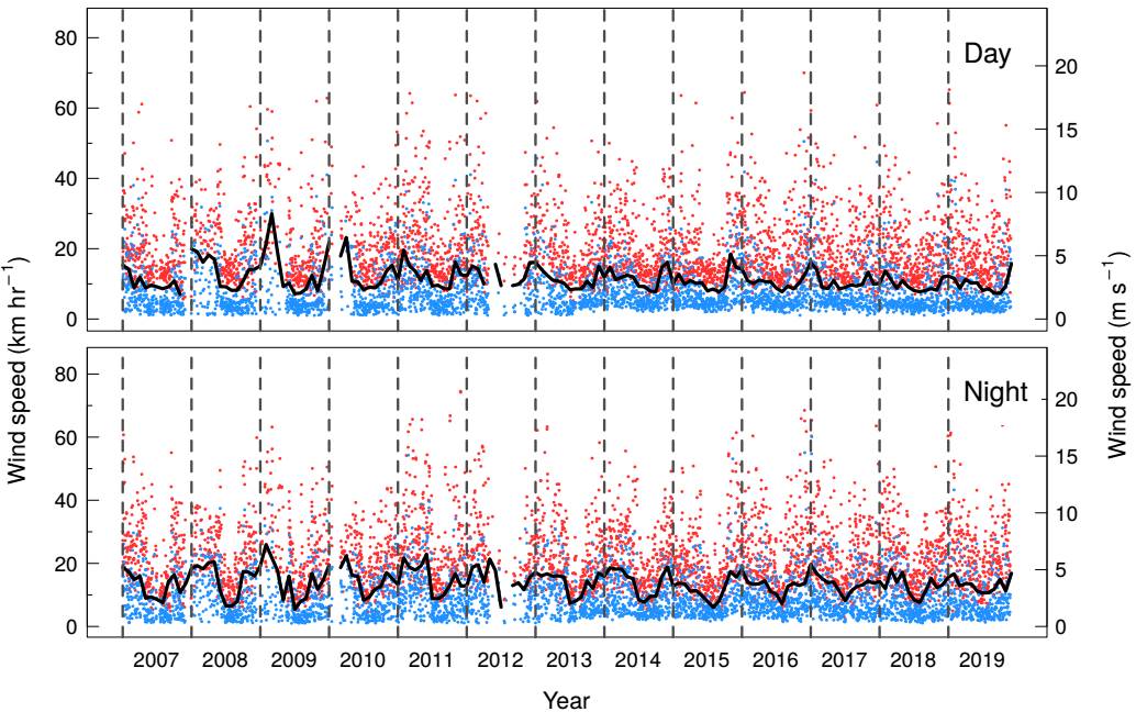
Fig. 18 We present the daily maximum (red) and minimum (blue) sustained wind speeds for daytime and nighttime data for the thirteen year time span of our data (2007-2019). In each panel the black line represents the median monthly wind speed and the vertical dashed lines indicate the first day of each year. These graphs include data from sites 1, 2 and 3. The color figure can be viewed online.
In Figure 19a and Table 16, we present the cumulative distribution of sustained wind and wind gust speeds for daytime and nighttime data. From this figure, it is clear that the wind speeds, both sustained and gusts, are stronger at night. The median sustained wind speed for daytime is 10.6km hr−1 (2.9m s−1) and at nighttime 12.9km hr−1 (3.6m s−1), while the median wind gust speeds are 20.1km hr−1 (5.6m s−1) and 21.5km hr−1 (≈6.0m s−1) for daytime and nighttime, respectively.
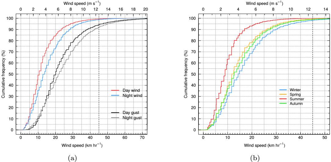
Fig. 19 We present (a) the cumulative distribution of the daytime and nighttime sustained wind speed and wind gusts for the period 2007-2019, based upon the 5 minute average and maximum values, respectively. The blue line stands for nighttime and the red line for daytime sustained wind data. The gray line stands for nighttime and the black line for daytime gusts wind data. In (b) we present the cumulative distribution of the sustained wind speed by season in the same period. The blue line stands for winter, the orange line for spring, the red line for summer and the green line for autumn. In both graphs, the dashed vertical line indicates the sustained wind speed limit of 45km hr−1 at which the domes of the OAN-SPM telescopes are closed. These graphs include data from sites 1, 2 and 3. The color figure can be viewed online.
The cumulative distributions for the speed of the daytime and nighttime sustained winds differ greatly in shape. In Figure 19a, we also indicate the speed limit of 45km hr−1 (12.5m s−1) for the sustained wind at which the OAN-SPM’s telescope domes are closed. The fraction of time with the sustained wind speed above this limit is 1.2% during nighttime or 51.1 hours per year (see Table 16).
In Figure 19b and Table 16, we present the cumulative distribution of sustained wind speed by season. From Figure 19b, it can be seen that the season with the strongest winds is winter, with a median value of 14.3km hr−1 (4.0m s−1), while for the summer season this value is 8.9km hr−1 (2.5m s−1). Spring and autumn have median values of 11.7km hr−1 (3.3m s−1) and 12.7km hr−1 (≈3.5m s−1), respectively.
TABLE 16 DISTRIBUTION OF SUSTAINED WIND AND WIND GUST SPEEDS
| Speed (km hr−1) | Wind | Gusts | Wind | |||||
|---|---|---|---|---|---|---|---|---|
| Day | Night | Day | Night | Winter | Spring | Summer | Autumn | |
| 5 | 0.1183 | 0.0958 | 0.0058 | 0.0126 | 0.0711 | 0.0909 | 0.1768 | 0.0893 |
| 10 | 0.4909 | 0.3555 | 0.1041 | 0.1229 | 0.3039 | 0.3943 | 0.6338 | 0.3707 |
| 15 | 0.7345 | 0.5795 | 0.3071 | 0.2830 | 0.5287 | 0.6514 | 0.8611 | 0.5994 |
| 20 | 0.8409 | 0.7268 | 0.4920 | 0.4234 | 0.6848 | 0.7816 | 0.9301 | 0.7480 |
| 25 | 0.9202 | 0.8551 | 0.6765 | 0.5873 | 0.8293 | 0.8861 | 0.9693 | 0.8709 |
| 30 | 0.9559 | 0.9194 | 0.7876 | 0.7106 | 0.9001 | 0.9388 | 0.9848 | 0.9294 |
| 35 | 0.9777 | 0.9603 | 0.8685 | 0.8139 | 0.9453 | 0.9723 | 0.9942 | 0.9650 |
| 40 | 0.9870 | 0.9754 | 0.9104 | 0.8734 | 0.9647 | 0.9841 | 0.9972 | 0.9792 |
| 45 | 0.9939 | 0.9883 | 0.9425 | 0.9202 | 0.9819 | 0.9938 | 0.9991 | 0.9897 |
| 50 | 0.9969 | 0.9939 | 0.9621 | 0.9488 | 0.9900 | 0.9974 | 0.9998 | 0.9944 |
| 55 | 0.9986 | 0.9972 | 0.9754 | 0.9671 | 0.9949 | 0.9992 | 1 | 0.9974 |
| 60 | 0.9993 | 0.9985 | 0.9843 | 0.9789 | 0.9974 | .0.9996 | ··· | 0.9986 |
| 65 | 0.9998 | 0.9995 | 0.9909 | 0.9872 | 0.9992 | 0.9999 | ··· | 0.9994 |
| 70 | 0.9999 | 0.9998 | 0.9946 | 0.9924 | 0.9997 | 1 | ··· | 0.9998 |
| 75 | 1 | 0.9999 | 0.9965 | 0.9951 | 0.9998 | ··· | ··· | 0.9999 |
| 80 | ··· | 1 | 0.9980 | 0.9971 | 0.9999 | ··· | ··· | 1 |
| 85 | ··· | ··· | 0.9990 | 0.9984 | 1 | ··· | ··· | ··· |
| 90 | ··· | ··· | 0.9994 | 0.9990 | ··· | ··· | ··· | ··· |
| 95 | ··· | ··· | 0.9997 | 0.9995 | ··· | ··· | ··· | ··· |
| 100 | ··· | ··· | 0.9998 | 0.9997 | ··· | ··· | ··· | ··· |
| 105 | ··· | ··· | 0.9999 | 0.9999 | ··· | ··· | ··· | ··· |
| 110 | ··· | ··· | 0.9999 | 0.9999 | ··· | ··· | ··· | ··· |
| 115 | ··· | ··· | 1 | 1 | ··· | ··· | ··· | ··· |
In Figure 20, we show the cumulative distribution of the difference between the wind gusts and sustained wind speeds. When compared to the sustained wind and wind gust speeds, we find that for50% of the time wind gusts are stronger than sustained winds by 8.1 (nighttime) and 8.9km hr−1 (daytime) (2.3 and 2.5m s−1). The difference between the wind gust and the sustained wind speeds rarely exceeds 20km hr−1 (5.6m s−1), which occurs for less than 6% of the time.
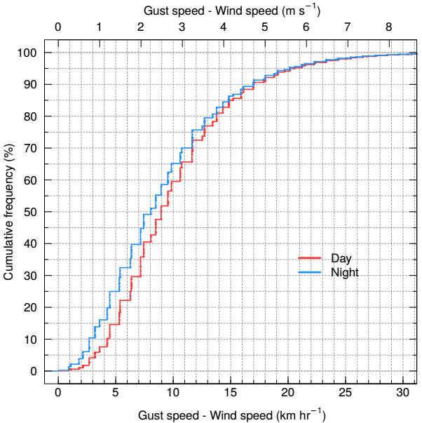
Fig. 20 We present the cumulative distribution of the daytime and nighttime difference between wind gust and sustained wind speeds for the period 2007-2019, based upon the 5 minute average and maximum values, respectively. The blue line stands for nighttime and the red line for daytime data. Values of the x-axis higher than 30km hr−1 represent less than 1% of the cases. This graph includes data from sites 1, 2 and 3. The color figure can be viewed online.
In Figure 21 we present hexagonal bin plots to show the distribution of values of the difference between wind gust and sustained wind speeds as a function of sustained wind speed for daytime and nighttime data. The color bar in the right part of each graph indicates the number of counts in each hexagonal bin. From Figure 21, it can be seen that given the limit of 45km hr−1 (12.5m s−1) in sustained wind speed, the corresponding wind gust speed will most probably be inside the range of 55-85km hr−1 (15.3-23.6m s−1).
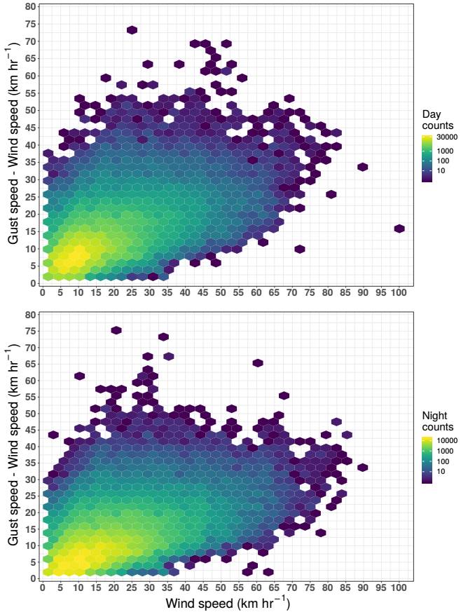
Fig. 21 We present hexagonal bin plots of the daytime (upper panel) and nighttime (bottom panel) difference between wind gust and sustained wind speeds as a function of sustained wind speed based upon the 5 minute average (sustained wind) and maximum (wind gust) values for the period 2007-2019. These graphs include data from sites 1, 2 and 3. The color figure can be viewed online.
Table 17 and Figure 24 present the monthly means of the sustained wind speed, where it can be seen that the strongest winds occur in December, January, February and March. Table 18 presents the dates with very strong sustained winds, defined as speeds ≥ 65km hr−1 (≥ 18m s−1) for more than 15 min. Most of the time, these very strong winds occur during November to February and come from SSW direction. Surprisingly, most of these events occurred during daytime. For these events, wind gust speeds usually are 20−30km hr−1 stronger than the sustained wind speed. The strongest wind gust speed registered is 129km hr−1 and it has been recorded four times since 2015, coming from SSW direction at night.
TABLE 17 MONTHLY MEAN SUSTAINED WIND AND WIND GUST SPEEDS
| Month | Day | Night Day | Night | |
|---|---|---|---|---|
| (km hr−1) | ||||
| January | 15 ± 10 | 17 ± 9 | 26 ± 14 | 27 ± 14 |
| February | 17 ± 10 | 19 ± 11 | 29 ± 15 | 30 ± 15 |
| March | 14 ± 10 | 18 ± 10 | 26 ± 14 | 28 ± 14 |
| April | 14 ± 8 | 17 ± 10 | 25 ± 12 | 27 ± 14 |
| May | 13 ± 8 | 16 ± 10 | 23 ± 11 | 25 ± 13 |
| June | 12 ± 7 | 15 ± 9 | 21 ± 10 | 23 ± 13 |
| July | 9 ± 5 | 9 ± 6 | 17 ± 7 | 16 ± 8 |
| August | 9 ± 5 | 10 ± 6 | 17 ± 7 | 17 ± 9 |
| September | 10 ± 6 | 12 ± 8 | 19 ± 10 | 20 ± 12 |
| October | 12 ± 8 | 15 ± 9 | 22 ± 12 | 24 ± 12 |
| November | 13 ± 9 | 16 ± 10 | 23 ± 13 | 25 ± 14 |
| December | 16 ± 10 | 17 ± 10 | 28 ± 15 | 28 ± 15 |
TABLE 18 HIGH WIND SPEEDSa
| Date | WindGustspeed | Winddirection | Time lapseb | |
|---|---|---|---|---|
| (km hr |
||||
| Dec 22, 2009 |
|
|
W | at 9:25-9:50 hrs |
| Nov 4, 2011 |
|
|
SSW | at 16:25-16:55 hrs |
| Jan 23, 2012 |
|
|
SSW | at 14:30-15:05 hrs |
| Dec 16, 2016 |
|
|
S | at 6:10-7:30 hrs |
| Feb 2, 2019 |
|
|
SSW | at 16:00-17:25 hrs |
| Feb 14, 2019 |
|
|
SSW | at 12:10-17:25 hrs |
Sustained wind speed ≥ 65km hr-1for more than 15 minutes.
Wind direction statistics are evaluated by calculating the percentage of the time in which the wind comes from each direction. The wind roses have been divided into sixteen mean directions. We have restricted sustained wind speed to values larger than or equal to 1km hr−1 (0.3m s−1), in order to obtain a set of wind direction values that is reliable. We tabulate lower wind speeds separately, without regard for their direction.
The wind roses of the sustained wind direction for daytime and nighttime are shown in Figures 22a and 22b, respectively. From this figure, there is little difference between daytime and nighttime in terms of wind direction. Taken as a whole, the predominant wind directions are SSW (202°±11°) and N (0°±11°). The wind rarely comes from the West or East. The strongest winds, those ≥45km hr−1, only come from South and SSW directions, while low speed winds mostly come from the North. Also, from Figures 22a and b it can be seen that high speed winds (≥20km hr−1) are more common at night, while low speed winds (5−20km hr−1) come during daytime.
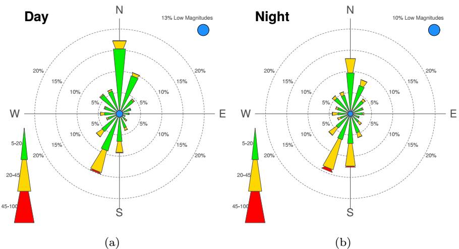
Fig. 22 We present wind roses (a) for daytime and (b) nighttime. The different colors within the roses indicate different velocity ranges. In the center of the wind roses, “low magnitudes” represent velocities in the range (1kmhr−1 - 5kmhr−1). The highest velocities, 45-100km hr−1 are represented in red color. The data used here are from sites 1 and 3. The color figure can be viewed online.
Since the wind direction is similar for daytime and night data, in the following we present only the nighttime wind roses. In Figure 23, we present the wind roses for each season. From this figure, it can be seen that during winter and spring the dominant wind direction is SSW direction (202°), and that the strongest winds (> 45km hr−1) also come from this direction. During the summer, there is a bipolar distribution of the winds, with North and South dominant directions, but no strong winds. Finally, in the autumn, most of the winds come from the North and some strong winds from the South and SSW direction.
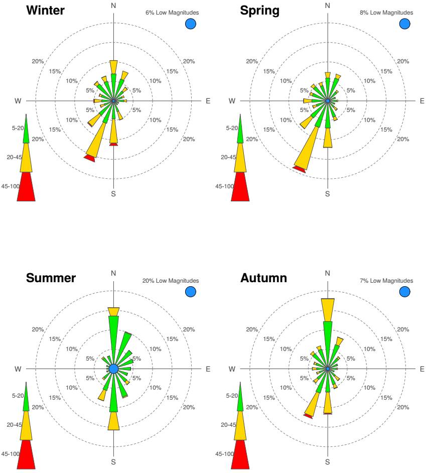
Fig. 23 We present nighttime wind roses for each season. The different colors within the roses indicate different velocity ranges. In the center of the wind roses, “low magnitudes” represent velocities in the range (1km hr−1 - 5km hr−1). The highest velocities, 45-100km hr−1 are represented in red color. The data used here are from sites 1 and 3. The color figure can be viewed online.
4. CONCLUSIONS
We analyze thirteen years of weather conditions at the Observatorio Astronómico Nacional in the Sierra San Pedro Mártir. The weather parameters we consider are: air temperature, relative humidity, atmospheric pressure, precipitation, sustained and wind gust speeds and direction. The data have been split in two sets, one for daytime and the other for nighttime. Figure 24 summarizes many of our results. Our main conclusions are:
Most of the time, the air temperature is below 15°C. The median temperature is 10.3°C and 7.0°C for daytime and nighttime, respectively, with a median diurnal variation of ∆T = 5.4°C. At night, the temperature is quite constant with a mean value of the rate of change of −0.06 ± 0.22°C per hour around midnight.
The coldest month is January with a mean temperature of 2.1°C and the warmest month is July with a mean temperature of 15.1°C. We searched for an increase in temperature over the last thirteen years and over the last 50 years (using data from Álvarez et al. 2007), but have not´ found any significant variation, at least at the 95% confidence level. Also, we have not found any increase in the number of warm days nor a decrease in the number of cold days over the thirteen years spanned by our data.
The relative humidity is statistically different for daytime and nighttime with median values of 30% and 27%, respectively. The diurnal variation of this parameter shows that the relative humidity is quite constant from midnight to sunrise, but that it varies during the rest of the day. The largest variations are found in spring and summer. The driest season is spring, with a median relative humidity of 23% while the most humid season is summer, with median relative humidity of 51%. We find no evidence for a long term evolution in the relative humidity over the time span of our data.
The median value of the atmospheric pressure is ≈730mb. During daytime, the atmospheric pressure is slightly higher than at night, by 0.5mb. This parameter varies seasonally, with the highest atmospheric pressure during summer. The diurnal variation of the atmospheric pressure is ≈ 2mb, due to the phenomenon known as atmospheric tides. On average, the atmospheric pressure has increased by 1mb in the last decade (95% confidence level).
The annual mean accumulated precipitation is ≈313mm, 70% of which occurs during summer time. Also, on average it rains four times more during the day than at night. However, our precipitation data for winter is an under-estimate of the true precipitation due to insensitivity of our sensors to frozen precipitation. Correcting for this, we estimate that the total annual precipitation at the OAN-SPM is 400-450 mm. The annual accumulated precipitation has increased over the time span of our data, with 30mm more precipitation every year since 2009 (99% confidence level).
The median value of the sustained wind speed is 11km hr−1 during the day and 13km hr−1 at night. The predominant wind directions are SSW (202°) and North (0°). The sustained wind is stronger at night, during the winter, and comes mainly from SSW direction. The median values of the wind gust speed are 20kmhr−1 and 22kmhr−1 for daytime and nighttime, respectively. Wind gust speeds are 9kmhr−1 stronger than sustained wind speeds 50% of the time. Only 5% of the time does the difference between wind gust and sustained wind speeds exceed 20kmhr−1.
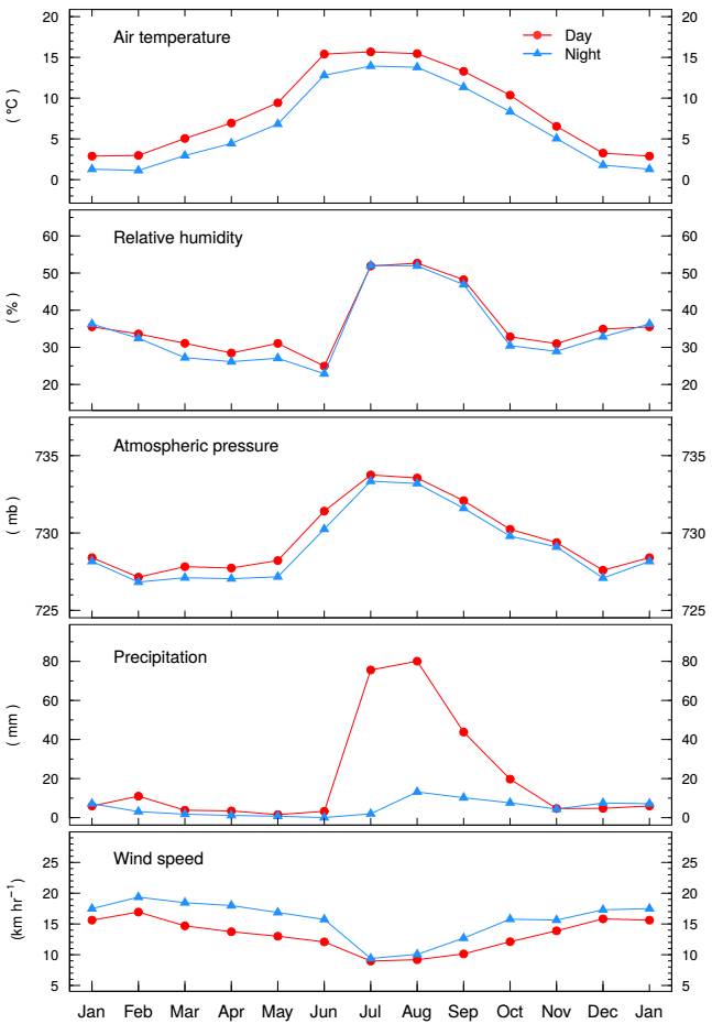
Fig. 24 We present the seasonal trends for (top to bottom) the mean air temperature, relative humidity, atmospheric pressure, precipitation, and sustained wind speed for daytime (circles/red) and nighttime (triangles/blue) for the period 2007-2019. The color figure can be viewed online.
We thank the anonymous referee for the careful reading and time spent to analyze this manuscript and the constructive comments and suggestions. This work is based upon observations carried out at the Observatorio Astronómico Nacional on the Sierra San Pedro Mártir (OAN-SPM), Baja California, México. We thank the daytime and night support staff at the OAN-SPM for facilitating and helping obtain these data: E. Cadena, T. Calvario, U. Ceseña, A. Córdova, A. Franco, B. García, F. Guillén, G. Guisa, J. Hernández, J. Herrera, D. Hiriart, E. López, B. Martínez, G. Melgoza, F. Montalvo, S. Monrroy, F. Murillo, C. Narváez, M. Núñez, J. L. Ochoa, F. Quiros, M. Reyes, H. Serrano, E. Valdés, J. Valdez, F. Valenzuela, I. Zavala and S. Zazueta. This paper is dedicated to the memory of our friends Gabriel Leyva Arias y Roberto Higuera Escalante.
Finally I. P-F. wants to acknowledge the use of the R package, which is a free software environment for statistical computing and graphics6.

