


 nueva página del texto (beta)
 Inglés (pdf)
 Artículo en XML
 Referencias del artículo
 Enviar artículo por email
 Citado por SciELO
  Similares en
SciELO
Similares en
SciELO 
 Permalink
1. INTRODUCTION
Astronomers have been trying to find a better way to understand stellar evolution in detail. Like the Kepler Mission, the space missions have been giving a new perspective on this point, as expected. For instance, the Kepler Mission first aimed to detect exo-planets (Borucki et al. 2010; Koch et al. 2010; Caldwell et al. 2010). For this aim, scientists counted on its highest quality and sensitivity ever obtained in the photometry (Jenkins et al. 2010a,b). Indeed, the high quality data accumulated by the Kepler Satellite revealed the presence of numerous variable targets, such as new eclipsing binaries, apart from discovering thousands of exo-planets (Slawson et al. 2011; Matijevič et al. 2012). Many of the newly discovered eclipsing binaries possess chromospherically active components (Balona 2015), while lots of them have pulsating components with several frequencies (Kamil and Dal 2017; Özdarcan and Dal 2017).
Stellar pulsation is an important phenomenon to understand stellar evolution. On this point, the very high precision photometry of the Kepler Satellite provides a remarkable chance to astronomers. Before the space missions, the photometric observations revealed the presence of several types of pulsating stars, such as γ Doradus, δ Scuti type pulsating, and also solar-like oscillating stars on the main sequence of the Hertzsprung-Russell (hereafter HR) diagram. Although there are several types of pulsating stars out of the main sequence, these samples are located close to the main sequence, sometimes side by side. In addition, the physical processes behind the pulsating nature of these stars are easily demonstrated by astroseismology, depending on the analysis of the pulsation frequencies. This is why the pulsating stars play a key role to understand stellar evolution (Cunha et al. 2007; Aerts et al. 2010).
Recent studies in the literature demonstrated that some stars can pulsate in both pressure (p) and gravity (g) modes. These stars are generally classified as γ Dor / δ Scuti hybrid pulsators. It is well known that p-modes, which are observed in the δ Scuti type variables, are generally sensitive to the outer layers of the star, while g-modes, which are observed in the γ Doradus type stars, are sensitive to the stellar interior (Aerts et al. 2010). After analyzing data obtained by the Kepler Satellite, the number of hybrid pulsators has remarkably increased (Grigahcéne et al. 2010; Uytterhoeven et al. 2011; Tkachenko et al. 2013; Balona 2014).
One of such systems worth examining is KIC 8043961 (Kirk et al. 2016), on which nature there are several debates. Although
there are several studies on KIC 8043961, they are generally grouped into two areas,
such as temperature and triplicity. Ammons et al.
(2006) computed the target
E(B−V ) as 0
m
.023 for its estimated distance of 76 pc. According to Pickles and Depagne (2010), KIC 8043961 is a main sequence
source of spectral type F6, while Watson et al.
(2006) listed the target as a variable star with a period of 1.559231 d.
They also gave the stellar distance as 589.757 pc depending on
Av
= 0
m
.358. Frasca et al. (2016) indicated
that the target was a main sequence source with a spectral type of F0F2. Some
physical parameters given in the literature are listed in Table 1 and, as seen from the table, the physical nature of
system is not absolutely determined. The most important study about KIC8043961 is
that of Conroy et al. (2014), where they
posited a third body in an almost circular orbit with period of 478 day, depending
on the eclipse time variation, and an amplitude of 184 s. Recently, Borkovits et al. (2016) also found a variation
with a period of 478.6 d from the eclipse times. Taking the total mass as
TABLE 1 LITERATURE PARAMETERS FOR THE TARGET
|
|
|
|
|
[Fe/H] | Ref |
|---|---|---|---|---|---|
| 6565 | - | - | - | 0.270 | Ammons et al. (2006) |
| 6348-6666 | 3.620 | - | - |
|
Pinsonneault et al. (2012) |
| 6657 | 3.621 | 3.177 | 1.532 |
|
Huber et al. (2014) |
| 6626-6935 | 4.100 | - | - |
|
Frasca et al. (2016) |
| 6649 | 3.619 | 3.177 | 1.532 |
|
Mathur et al. (2017) |
In this study, we try to reveal the nature of KIC 8043961, separately analyzing each variation detected in its light curve together with spectroscopic observations. In the next section, we summarize the observations and data reductions. Then, we determine the radial velocity variation from the available spectroscopic observations in § 3.1; we estimate the temperatures of the components from the same observations in § 3.2. To determine the size of the third body, we examine the O − C variation in § 3.3, and we model the light curve of the eclipsing binary in § 3.4. In § 3.5 we further analyse the out-of-eclipse variations. We summarize and discuss our findings in the last section.
2. OBSERVATIONS AND DATA REDUCTIONS
2.1. Spectral Observation
We carried out spectroscopic observations of the system with the 1.5-m Russian - Turkish telescope and the Turkish Faint Object Spectrograph Camera (TFOSC1) at Tubitak National Observatory. Using the échelle mode of TFOSC, we achieve an actual resolution of R=λ/∆λ ≈ 3000 around 5500Å. The whole spectrum covers a wavelength interval between 3900 - 9100Å in 11 échelle orders. All spectra were recorded with a back illuminated 2048 × 2048 pixels CCD camera, which has a pixel size of 15 × 15 µm 2.
We recorded eight optical spectra of KIC8043961 between the 2014 and 2017 observing seasons. In addition, we obtained optical spectra of ι Psc (HD 222368, F7V, vr = 5.656 kms−1) and o Aql (F8V, vr = 1.40 kms−1) with the same instrumental set-up. The spectra of these two stars were used as templates for radial velocity determinations and preliminary spectral type estimations. Typical signalto-noise ratios (SNR) of observed spectra are between 140 and 190 for a single observation with an hour of exposure time.
We reduced and extracted the observed spectra by following standard steps for reducing and extracting échelle spectra. In the first step, bias correction was applied to all images, and a normalized flatfield image was obtained via bias-corrected halogen lamp frames. Then, all science and Fe-Ar calibration frames were divided by the normalized flat-field frame; scattered light correction was applied to all bias and flat-field corrected images. At that point, reduced science and Fe-Ar images were obtained. Next, spectra were extracted from the reduced images. In the following steps, wavelength calibration was applied to the reduced and extracted science frames via Fe-Ar images, and finally wavelength calibrated science images were normalized to the continuum by using cubic spline functions. The whole procedure was applied under IRAF2 environment.
2.2. Photometric Data
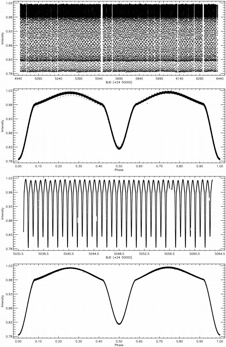
In the light curve and O−C analyses, we mainly use long cadence (29.4 minutes of exposure time, hereafter LC) Kepler photometry, which is available in the Kepler eclipsing binary catalogue3 as detrended and normalized fluxes (Slawson et al. 2011; Prša et al. 2011). We also use the short cadence (hereafter SC) data from the same database in the same format, in order to investigate possible high frequency variations. The data were collected over a broad wavelength interval between 4100Å and 9100Å, which suffers from lack of color information, but provides very high precision. The LC data cover ≈ 4 years of time base without any considerable time gap. The reported light contamination is 0.3% in the MAST database, practically meaning no light contribution of any light sources from the background. Available SC and LC photometry is shown in Figure 1. In the figure, we computed the phase-folded light curve with respect to the light elements in equation (1) given by Slawson et al. (2011).
3. ANALYSES AND MODELS
3.1. Radial Velocities and Spectroscopic Orbit
We start our analysis with the measurement of the radial velocities of each component, in order to determine the spectroscopic orbit of the system. For this purpose, we cross-correlate each observed spectrum of KIC 8043961 with spectra of ι Psc and o Aql. The cross correlation was applied according to the method proposed by Tonry and Davis (1979). The practical application of the method was done with the FXCOR task under IRAF environment. Among the two template stars, ι Psc provided a slightly better cross-correlation and was adopted as the radial velocity template. Cross-correlation was performed for the wavelength range between 4900 - 5400Å, ignoring strongly blended spectral lines. In Figure 2, we show the cross-correlation functions of spectra obtained at orbital quadratures, where both components are clearly resolved.
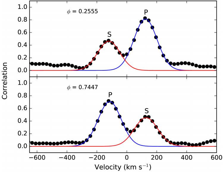
Fig. 2 Cross-correlation functions of KIC 8043961 obtained at orbital quadratures. The letter φ shows the orbital phase in each panel. P and S denote the primary and secondary component, respectively. The color figure can be viewed online.
We tabulate the measured radial velocities in Table 2, together with brief observational information. In the table, orbital phases are calculated via ephemeris time and period given by Borkovits et al. (2016). These light elements are adopted for phasing the radial velocities and light curve.
TABLE 2 SPECTROSCOPIC OBSERVATIONS AND RADIAL VELOCITIES
| HJD | Orbital | Exposure | Primary | Secondary | ||
|---|---|---|---|---|---|---|
| (24 00000+) | Phase | time (s) | V |
|
V |
|
| 56842.3645 | 0.7447 | 3000 |
|
11.3 | 109.3 | 19.8 |
| 56842.4005 | 0.7678 | 3000 |
|
6.9 | 115.0 | 13.3 |
| 56846.3781 | 0.3188 | 3000 | 91.3 | 10.3 |
|
21.6 |
| 56888.2869 | 0.1970 | 3000 | 98.3 | 9.0 |
|
19.8 |
| 56891.4965 | 0.2555 | 3000 | 108.0 | 6.9 |
|
17.7 |
| 57592.4858 | 0.8344 | 1200 |
|
10.3 | 113.5 | 19.3 |
| 57616.3579 | 0.1448 | 3600 | 73.2 | 10.1 |
|
26.0 |
| 57854.5254 | 0.8934 | 2700 |
|
15.0 | 48.9 | 25.9 |
Before attempting an orbital solution, we inspected the orbital eccentricity via phased folded Kepler photometry. Primary and secondary eclipses are located precisely at 0.0 and 0.5 phases, respectively, indicating a non-eccentric orbit. Therefore, we model the spectroscopic orbit assuming a circular orbit. The orbital solution was achieved by applying the Levenberg-Marquardt algorithm (Levenberg 1944), and Markov Chain Monte Carlo simulations via EMCEE software developed under a Python environment (Foreman-Mackey et al. 2013). We tabulate the final spectroscopic orbit parameters and their uncertainties in Table 3, and we plot the phasefolded radial velocities, theoretical models and residuals from the best-fitting models in Figure 3. We notice that the less massive, smaller and hotter component is eclipsed at the primary minimum, hence we interpret the numerical values in Table 3 according to this finding.
TABLE 3 SPECTROSCOPIC ORBITAL ELEMENTS OF KIC8043961*
| Parameter | Value |
|---|---|
| Porb (days) | 1.5592121 (fixed) |
| T0 (HJD2454+) | 954.555903 (fixed) |
|
|
|
|
|
|
|
|
|
|
|
0 (fixed) |
|
|
… |
|
|
|
|
|
|
| Mass ratio
( |
|
| rms1 (km
s |
3.4 |
| rms2 (km s |
8.9 |
* M1 and M2, masses of the primary and secondary component, M the total mass of the system.

3.2. Spectral Type
In order to estimate atmospheric properties of the components reliably, we use the TFOSC spectrum of KIC 8043961 obtained at HJD 2456842.3645, corresponding to ≈ 0.75 orbital phase, where we can clearly resolve spectral lines of both components. The SNR of that spectrum is around 170, based on photon statistics. Before searching for the best atmospheric parameters, we fixed the micro-turbulence velocity of each component at 2 kms−1, and the logarithm of the surface gravity log(g) of the primary and secondary components at 4.04 and 3.77, respectively. These log(g) values are calculated from combination of spectroscopic orbit parameters and light curve modeling results (see next section). Then we adjusted effective temperatures and metallicities of the components via the spectral synthesis method in a wavelength interval 4750 - 5750Å. In practice, we used the latest version of the Python framework iSpec (Blanco-Cuaresma et al. 2014). Synthetic spectra were calculated for temperatures between 6250 - 7250 K with steps of 50 K, and for metallicities between solar (0.0) and −1.0 with steps of 0.25. Among the different radiative transfer code options provided by iSpec, we adopted SPECTRUM4 code (Gray and Corbally 1994) along with ATLAS9 model atmospheres (Castelli and Kurucz 2004) and a line list obtained from the third version of the Vienna atomic line database (VALD3) (Ryabchikova et al. 2015).
All calculated synthetic spectra were convolved with a Gaussian line spread function to match their resolution to the TFOSC spectra. After we obtained the instrumentally broadened synthetic spectra, we started to calculate the composite spectrum of the system. At that point, we selected a trial synthetic spectrum for the primary component. Next, we selected a synthetic spectrum for the secondary component, with a proper temperature as indicated by the preliminary light curve modelling. Then, we applied a proper radial velocity shift to each selected synthetic spectrum to match its spectral lines to the lines of the corresponding component in the observed spectrum. Finally, we calculated the composite spectrum of the system via synthetic spectra mentioned above, and the radius ratio, R1 /R2 = r1 /r2 = 0.69, where r means fractional radius, found from the light curve analysis. We repeated this process for every possible synthetic spectra configuration and searched the best matched composite spectrum of the system, i.e. the best-fitting synthetic spectrum for each component. We checked the reliability of the parameters suggested by the best matched synthetic spectra, with the best-fitting light curve model parameters. Confirming the light curve and spectroscopic modelling results iteratively, we find the selfconsistent effective temperature of the primary and the secondary component as 6900 K and 6600 K. The temperatures and the surface gravities suggest F3V and F5 III-IV spectral types for the hot and cool components, respectively (Gray 2005). The resulting overall metallicity of the system is found to be [M/H] = 0.25. Estimated uncertainties are 200K in temperature and -0.25 in metallicity, which are predicted by considering the temperature and metallicity steps in the model atmospheres, the SNR of observed spectra and the instrumental resolution of TFOSC spectra.
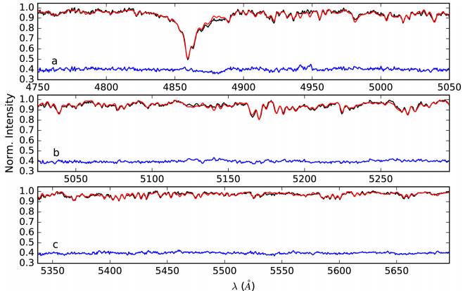
Furthermore, we observe a perceivable effect of rotational broadening in our spectra. Full width at half-maximum (FWHM) of the instrumental profile of TFOSC spectra is ≈1.8Å around 5500 Å, meaning that any projected rotational velocities (v sini) above ≈ 50 km s−1could be observed. From the combined spectroscopic orbit and light curve modelling, we estimate v sini values of the primary and the secondary component as 81 km s−1and 54 km s−1, respectively, assuming synchronous rotation. Since numerical fitting attempts of v sini velocities did not yield stable and reliable results, we only applied rotational broadening to the corresponding synthetic spectrum of the components, by using the estimated velocities above, and then calculated the composite spectrum of the system. In Figure 4, we plot observed spectrum, best fitting composite synthetic spectrum and residuals.
3.3. Orbital Period Variation
In order to study the orbital period variation of KIC 8043961, we determine mid-times of primary and secondary eclipses, where we obtain 1688 minima times in total, of which 844 are the primary minima and 844 the secondary times of minimum. For each minimum, we only consider the orbital cycle that includes the corresponding minimum, and
then run the differential correction program of the Wilson-Devinney code by only adjusting ephemeris time and keeping all other parameters fixed. This process is fairly straightforward for primary eclipses, while we need to change the role of the components during the iterations, in order to compute secondary eclipses. Ten computed minima times are listed in Table 4, while the rest of them are available upon request. For each observed eclipse time, we compute expected eclipse times by using the following light elements (equation 1) to obtain O − C values:
TABLE 4 TIMES OF MINIMA AND O − C RESIDUALS*
| MJD (Obs) | E | Type | O-C (II) (day) |
|---|---|---|---|
| 54953.77420 | −0.5 | II | −0.00141 |
| 54954.55380 | 0.0 | I | −0.00142 |
| 54955.33380 | 0.5 | II | −0.00103 |
| 54956.11340 | 1.0 | I | −0.00103 |
| 54956.89260 | 1.5 | II | −0.00144 |
| 54957.67220 | 2.0 | I | −0.00145 |
| 54958.45190 | 2.5 | II | −0.00135 |
| 54959.23150 | 3.0 | I | −0.00136 |
| 54960.01120 | 3.5 | II | −0.00127 |
| 54960.79080 | 4.0 | I | −0.00127 |
*Obtained from the Kepler SC and LC data.
Inspecting the O − C values, we notice a clear sinusoidal variation, which is presumably due to the light travel time effect (hereafter LTTE) caused by an unseen third body in the system. Taking the light elements given in equation (1) as initial values, we modelled the sinusoidal variation together with the linear trend. Corrected ephemeris time and period are given by equation (2):
where ∆t is term for the LTTE of the third body. Using the corrected ephemeris time and the period, we calculate (O−C) II residuals. Applying the LTTE equation given by Irwin (1959) to the (O−C) II residuals, we calculate the orbit of the third body. In Figure 5, we show (O−C) II residuals together with the best-fitting third body orbit. Calculated third body parameters are listed in Table 5.
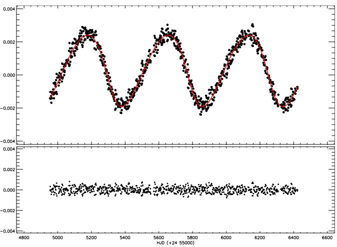
Fig. 5 The O-C variations of KIC 8043961. In the figure, the (O-C) II variation, derived after the linear correction, is shown in the upper panel, together with the best-fitting orbit (smooth red curve), while the residuals are shown in the bottom panel. The color figure can be viewed online.
TABLE 5 THIRD BODY PARAMETERS OF KIC 8043961*
|
|
|
|
|
|
|
|
|
|
|
|
|
|
|
|
|
|
|
|
|
|
|
4.909 (for
|
|
|
1.161 (for
|
|
|
0.799 (for
|
|
|
0.767 (for |
* Derived from O-C analysis.
Assuming that the orbital inclination of the presumed third body is the same as
the inclination of the eclipsing binary, and using the calculated total mass of
the eclipsing binary (2.892
3.4. Light Curve Analysis
To determine the physical conditions of the components, we model the average SC light curve by using 2015 version of the Wilson - Devinney Code (Wilson and Devinney 1971; Wilson and Van Hamme 2014). The shape of the light curve clearly indicates a detached configuration. In the analysis, we fix the two critical parameters, mass ratio and effective temperature of the primary component (T1) to 1.09 and 6900 K, respectively, which are found from the spectroscopic orbit modelling and the spectral type estimation. Considering the spectral type corresponding to this temperature, the albedos (A1 and A2) and the gravity-darkening coefficients (g1 and g2) of the components are adopted for the stars with convective envelopes (Lucy 1967; Rucinski 1969). The nonlinear limb-darkening coefficients (x1 and x2) of the components are taken from Van Hamme (1993). In the analyses, the temperature of the secondary component (T2), the dimensionless potentials of the components (Ω1 and Ω2), the fractional luminosity of the primary component (L1), the inclination of the system (i), the mass ratio of the system (q), the semi-major axis (a) and the third light are adopted as adjustable parameters. Although the synthetic curve derived by these parameters covers the entire observed light curve, a stable sinusoidal variation is still seen at out-of-eclipses. Considering the temperatures of the components, we modelled this variation by a stellar cool spot on the secondary component. We list the best-fitting model results in Table 6, and show the averaged phase-folded light curve together with the model in Figure 6.
TABLE 6 LIGHT CURVE MODELLING RESULTS FOR KIC 8043961*
| Parameter | Value |
|---|---|
| q | 1.09 ± 0.07 |
| i (◦) | 73.71 ± 0.02 |
| T1 (K) | 6900 (fixed) |
| T2 (K) | 6598 ± 200 |
| Ω1 | 5.581 ± 0.003 |
| Ω2 | 4.432 ± 0.002 |
| L1/LT | 0.3450 ± 0.0005 |
| L2/LT | 0.6008 |
| L3/LT | 0.0542 ± 0.0012 |
| g1, g2 | 0.32 (fixed), 0.457 ± 0.007 |
| A1, A2 | 0.50 (fixed), 0.451 ± 0.003 |
| x1, x2 | 0.654, 0.663 (fixed) |
| y1, y2 | 0.283, 0.274 (fixed) |
| < r1 > | 0.2261 ± 0.0001 |
| < r2 > | 0.3286 ± 0.0002 |
| Phase Shift | −0.000208 ± 0.000009 |
| Co − LatSpotI (rad) | 1.519 ± 0.118 |
| LongSpotI (rad) | 1.808 ± 0.021 |
| RSpotI (rad) | 0.183 ± 0.004 |
| TfSpotI | 0.98 (fixed) |
*Internal uncertainty of T2 is found as a few Kelvin, which is unrealistic, therefore it is assumed to be the same as the uncertainty of T1.
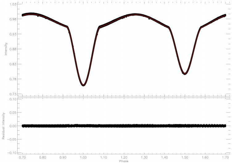
Fig. 6 Phase-folded LC light curve (filled circles) taken from the Kepler Database, and the best-fitting model (smooth red curve). The color figure can be viewed online.
The combination of results obtained from both the spectroscopic orbit and light
curve modelling yields the physical parameters of the system listed in Table 7. These parameters show that the
smaller, hotter and less massive primary component is still on the main
sequence, while the larger, cooler and more massive secondary component appears
to have evolved off the main sequence. We show the position of the components on
the log
TABLE 7 PHYSICAL PARAMETERS OF KIC 8043961
| Parameter | Primary | Secondary |
|---|---|---|
| Mass ( |
1.379 |
1.513 |
| Separation
( |
8.06 |
|
| Radius ( |
1.806 |
2.611 |
|
|
0.833 |
1.075 |
|
|
4.06 |
3.78 |
|
|
2.70 |
2.10 |
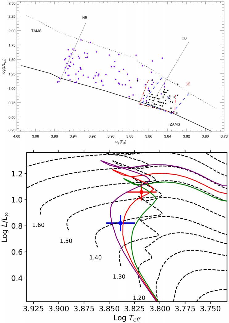
Fig. 7 Upper panel. Positions of the primary (blue asterisk) and the
secondary (red asterisk) components of KIC 8043961 on the
3.5. The Variation at Out-Of-Eclipses
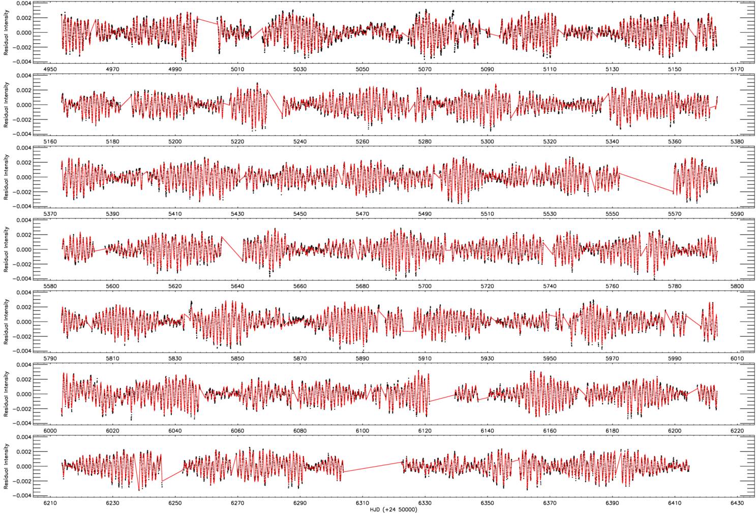
Inspecting the residuals from the light curve modeling, we find a clear signal of a sinusoidal variation at out-of-eclipses. Considering the place of the primary component of KIC 8043961 in the HR diagram, the source of the variation is possibly a γ Doradus type pulsation. We analyse the residual data to search for possible pulsation frequencies, using the PERIOD04 software (Lenz and Breger 2005) that is based on the discrete Fourier transform (hereafter DFT) method (Scargle 1982). As seen in Figure 8, we found 137 frequencies which exceed the 3 σ level. We tabulate these frequencies in Table 8, and plot the resulting model obtained from these frequencies together with the residual light curve in Figure 9.
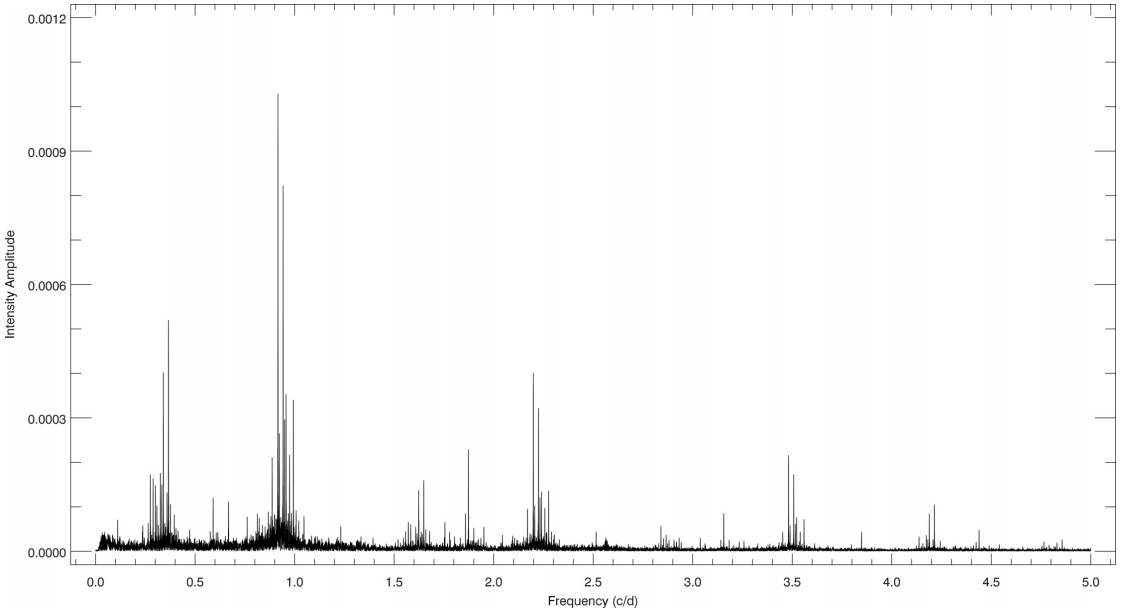
TABLE 8 FREQUENCY LIST OF γ DOR PULSATION FOUND IN THE ANALYSIS*
| Frequency | Frequency | Amplitude | Phase | Noise | SNR |
|---|---|---|---|---|---|
| F1 | 0.916416 | 0.000975 | 0.976502 | 0.000015 | 69.954572 |
| F2 | 0.942190 | 0.000792 | 0.568788 | 0.000012 | 67.223506 |
| F3 | 0.956949 | 0.000353 | 0.562851 | 0.000011 | 31.818026 |
| F4 | 0.993697 | 0.000308 | 0.028697 | 0.000010 | 30.623664 |
| F5 | 0.949851 | 0.000273 | 0.393345 | 0.000010 | 28.959837 |
| F6 | 0.923608 | 0.000243 | 0.363458 | 0.000010 | 26.495071 |
| F7 | 1.873358 | 0.000231 | 0.189382 | 0.000005 | 50.902279 |
| F8 | 0.974498 | 0.000216 | 0.338794 | 0.000009 | 25.021613 |
| F9 | 0.887055 | 0.000210 | 0.765381 | 0.000008 | 25.319987 |
| F10 | 0.275072 | 0.000177 | 0.791680 | 0.000010 | 16.599333 |
| F11 | 0.300848 | 0.000144 | 0.306613 | 0.000009 | 15.496189 |
| F12 | 0.668357 | 0.000113 | 0.388377 | 0.000007 | 16.524546 |
| F13 | 0.366276 | 0.000130 | 0.127347 | 0.000008 | 15.950863 |
| F14 | 0.376595 | 0.000111 | 0.761279 | 0.000008 | 13.586635 |
| F15 | 0.984063 | 0.000092 | 0.535489 | 0.000008 | 12.104475 |
| F16 | 1.858608 | 0.000087 | 0.763904 | 0.000004 | 21.211509 |
| F17 | 0.868183 | 0.000091 | 0.198983 | 0.000007 | 11.746275 |
| F18 | 1.047241 | 0.000076 | 0.320245 | 0.000007 | 10.264264 |
| F19 | 0.761510 | 0.000070 | 0.821559 | 0.000007 | 10.089111 |
| F20 | 0.881004 | 0.000068 | 0.608747 | 0.000007 | 10.238665 |
| F21 | 0.931190 | 0.000072 | 0.225136 | 0.000007 | 10.314234 |
| F22 | 0.822440 | 0.000072 | 0.054409 | 0.000007 | 10.020085 |
| F23 | 0.838783 | 0.000065 | 0.057601 | 0.000007 | 10.032803 |
| F24 | 1.755210 | 0.000077 | 0.656801 | 0.000004 | 15.728606 |
| F25 | 0.813057 | 0.000071 | 0.114027 | 0.000007 | 9.982051 |
| F26 | 0.111354 | 0.000066 | 0.958094 | 0.000010 | 6.260455 |
| F27 | 0.340336 | 0.000079 | 0.796978 | 0.000008 | 9.859690 |
| F28 | 1.232040 | 0.000081 | 0.621758 | 0.000007 | 9.553888 |
| F29 | 1.571022 | 0.000063 | 0.671356 | 0.000005 | 13.521431 |
| F30 | 0.264255 | 0.000068 | 0.477712 | 0.000009 | 6.833383 |
| F31 | 0.965094 | 0.000059 | 0.188122 | 0.000007 | 8.480951 |
| F32 | 0.899936 | 0.000063 | 0.045391 | 0.000007 | 8.709595 |
| F33 | 0.315615 | 0.000067 | 0.768945 | 0.000008 | 6.948675 |
| F34 | 0.237268 | 0.000058 | 0.947569 | 0.000009 | 5.865668 |
| F35 | 0.404073 | 0.000055 | 0.148505 | 0.000007 | 8.085690 |
| F36 | 0.348656 | 0.000050 | 0.010840 | 0.000007 | 7.620083 |
| F37 | 0.836521 | 0.000051 | 0.294970 | 0.000006 | 8.112678 |
| F38 | 0.943443 | 0.000049 | 0.595186 | 0.000006 | 7.689664 |
| F39 | 1.557797 | 0.000058 | 0.084863 | 0.000004 | 13.069212 |
| F40 | 1.900344 | 0.000049 | 0.169896 | 0.000004 | 13.102947 |
| F41 | 1.624016 | 0.000048 | 0.644379 | 0.000004 | 11.457698 |
| F42 | 0.352339 | 0.000053 | 0.656969 | 0.000007 | 7.038268 |
| F43 | 1.778928 | 0.000043 | 0.665775 | 0.000004 | 11.216445 |
| F44 | 0.050852 | 0.000050 | 0.030521 | 0.000011 | 4.903525 |
| F45 | 0.606112 | 0.000048 | 0.492856 | 0.000006 | 8.230251 |
| F46 | 1.636105 | 0.000045 | 0.454696 | 0.000004 | 11.144403 |
| F47 | 0.045897 | 0.000046 | 0.610881 | 0.000011 | 4.116043 |
| F48 | 0.332966 | 0.000054 | 0.719763 | 0.000007 | 7.587804 |
| F49 | 0.969087 | 0.000040 | 0.442950 | 0.000006 | 6.680742 |
| F50 | 0.033530 | 0.000040 | 0.260326 | 0.000011 | 3.946902 |
| F51 | 0.041740 | 0.000047 | 0.429774 | 0.000011 | 4.078355 |
| F52 | 0.062306 | 0.000037 | 0.493489 | 0.000010 | 4.169141 |
| F53 | 0.923070 | 0.000043 | 0.116737 | 0.000006 | 7.247459 |
| F54 | 3.848074 | 0.000041 | 0.054995 | 0.000002 | 26.143136 |
| F55 | 0.875308 | 0.000042 | 0.639336 | 0.000006 | 6.855955 |
| F56 | 0.899008 | 0.000044 | 0.795619 | 0.000006 | 7.304526 |
| F57 | 0.035574 | 0.000044 | 0.888834 | 0.000011 | 3.755091 |
| F58 | 0.893106 | 0.000039 | 0.673879 | 0.000006 | 6.583598 |
| F59 | 0.071598 | 0.000043 | 0.565349 | 0.000010 | 3.878613 |
| F60 | 1.217177 | 0.000035 | 0.448149 | 0.000006 | 6.225868 |
| F61 | 1.113841 | 0.000039 | 0.919774 | 0.000006 | 6.361630 |
| F62 | 0.084857 | 0.000036 | 0.273882 | 0.000010 | 3.841943 |
| F63 | 0.862411 | 0.000036 | 0.413632 | 0.000006 | 6.209853 |
| F64 | 0.308531 | 0.000042 | 0.978470 | 0.000007 | 5.737678 |
| F65 | 0.039757 | 0.000037 | 0.482542 | 0.000010 | 3.592632 |
| F66 | 0.086183 | 0.000044 | 0.204570 | 0.000010 | 3.904434 |
| F67 | 0.028510 | 0.000036 | 0.522162 | 0.000010 | 3.593336 |
| F68 | 0.037625 | 0.000033 | 0.879902 | 0.000010 | 3.707129 |
| F69 | 0.066868 | 0.000036 | 0.694784 | 0.000010 | 3.749136 |
| F70 | 0.833279 | 0.000034 | 0.689229 | 0.000006 | 6.115674 |
| F71 | 1.935889 | 0.000034 | 0.797306 | 0.000003 | 10.342439 |
| F72 | 0.046928 | 0.000033 | 0.926278 | 0.000010 | 3.641927 |
| F73 | 0.752865 | 0.000032 | 0.937067 | 0.000006 | 5.713433 |
| F74 | 0.282383 | 0.000036 | 0.613151 | 0.000007 | 4.667376 |
| F75 | 0.072970 | 0.000028 | 0.029980 | 0.000009 | 3.490809 |
| F76 | 0.810075 | 0.000034 | 0.929619 | 0.000006 | 5.908784 |
| F77 | 1.040132 | 0.000031 | 0.368693 | 0.000006 | 5.415959 |
| F78 | 1.583709 | 0.000039 | 0.872553 | 0.000004 | 9.394488 |
| F79 | 0.118384 | 0.000038 | 0.211363 | 0.000009 | 3.530131 |
| F80 | 0.122063 | 0.000033 | 0.274277 | 0.000009 | 3.576727 |
| F81 | 0.044769 | 0.000031 | 0.735394 | 0.000010 | 3.384484 |
| F82 | 0.805382 | 0.000030 | 0.060741 | 0.000006 | 5.294651 |
| F83 | 0.780749 | 0.000031 | 0.365751 | 0.000006 | 5.371773 |
| F84 | 1.020802 | 0.000027 | 0.375184 | 0.000006 | 5.185010 |
| F85 | 0.846646 | 0.000030 | 0.693919 | 0.000006 | 5.545416 |
| F86 | 0.043761 | 0.000034 | 0.107477 | 0.000009 | 3.412263 |
| F87 | 0.034585 | 0.000039 | 0.200139 | 0.000010 | 3.459900 |
| F88 | 0.245707 | 0.000031 | 0.792545 | 0.000007 | 4.078792 |
| F89 | 0.067848 | 0.000035 | 0.019685 | 0.000009 | 3.554611 |
| F90 | 0.359000 | 0.000035 | 0.418093 | 0.000006 | 6.172003 |
| F91 | 0.088419 | 0.000031 | 0.117918 | 0.000009 | 3.347851 |
| F92 | 0.049519 | 0.000031 | 0.486309 | 0.000009 | 3.294346 |
| F93 | 0.063776 | 0.000033 | 0.104108 | 0.000009 | 3.338091 |
| F94 | 2.562753 | 0.000026 | 0.981644 | 0.000003 | 8.832871 |
| F95 | 1.050964 | 0.000028 | 0.679146 | 0.000006 | 5.069696 |
| F96 | 0.120176 | 0.000027 | 0.035077 | 0.000008 | 3.521058 |
| F97 | 1.832863 | 0.000027 | 0.560490 | 0.000003 | 8.258790 |
| F98 | 0.054958 | 0.000026 | 0.032402 | 0.000009 | 3.240881 |
| F99 | 0.818258 | 0.000029 | 0.418968 | 0.000005 | 5.095555 |
| F100 | 0.032542 | 0.000031 | 0.505786 | 0.000009 | 3.299345 |
| F101 | 0.061774 | 0.000029 | 0.393201 | 0.000009 | 3.545683 |
| F102 | 2.304441 | 0.000028 | 0.820278 | 0.000003 | 9.129813 |
| F103 | 1.916937 | 0.000027 | 0.628618 | 0.000003 | 8.333952 |
| F104 | 1.017917 | 0.000028 | 0.195242 | 0.000006 | 4.844850 |
| F105 | 0.122733 | 0.000029 | 0.432214 | 0.000008 | 3.368645 |
| F106 | 0.950408 | 0.000028 | 0.602112 | 0.000005 | 5.224705 |
| F107 | 0.821818 | 0.000027 | 0.269326 | 0.000005 | 4.904104 |
| F108 | 0.841843 | 0.000026 | 0.694110 | 0.000005 | 4.802736 |
| F109 | 0.829256 | 0.000026 | 0.364050 | 0.000005 | 4.815170 |
| F110 | 1.924095 | 0.000026 | 0.710283 | 0.000003 | 8.248569 |
| F111 | 1.803526 | 0.000026 | 0.101545 | 0.000003 | 7.742789 |
| F112 | 0.110544 | 0.000026 | 0.860448 | 0.000008 | 3.174831 |
| F113 | 0.121371 | 0.000028 | 0.336842 | 0.000008 | 3.299731 |
| F114 | 0.667256 | 0.000026 | 0.971549 | 0.000005 | 5.183159 |
| F115 | 1.085479 | 0.000025 | 0.856127 | 0.000005 | 4.717625 |
| F116 | 0.078042 | 0.000026 | 0.774947 | 0.000008 | 3.147375 |
| F117 | 0.139951 | 0.000025 | 0.056737 | 0.000008 | 3.302504 |
| F118 | 0.879551 | 0.000025 | 0.330724 | 0.000005 | 4.705819 |
| F119 | 0.325674 | 0.000030 | 0.500824 | 0.000006 | 4.975161 |
| F120 | 0.289150 | 0.000028 | 0.489091 | 0.000006 | 4.504696 |
| F121 | 0.097427 | 0.000026 | 0.330393 | 0.000008 | 3.024391 |
| F122 | 0.183915 | 0.000024 | 0.516818 | 0.000007 | 3.389604 |
| F123 | 0.679402 | 0.000023 | 0.754883 | 0.000005 | 4.665421 |
| F124 | 0.785210 | 0.000024 | 0.650818 | 0.000005 | 4.493476 |
| F125 | 0.349622 | 0.000024 | 0.885464 | 0.000005 | 4.458943 |
| F126 | 0.976807 | 0.000023 | 0.012797 | 0.000005 | 4.546269 |
| F127 | 0.826710 | 0.000023 | 0.947968 | 0.000005 | 4.591718 |
| F128 | 0.135705 | 0.000023 | 0.926925 | 0.000007 | 3.195712 |
| F129 | 0.073810 | 0.000025 | 0.799563 | 0.000008 | 3.098061 |
| F130 | 0.096326 | 0.000025 | 0.795353 | 0.000008 | 3.195557 |
| F131 | 0.065866 | 0.000026 | 0.081159 | 0.000008 | 3.400311 |
| F132 | 2.568079 | 0.000022 | 0.918795 | 0.000003 | 7.820700 |
| F133 | 0.124682 | 0.000023 | 0.168908 | 0.000007 | 3.082160 |
| F134 | 0.850509 | 0.000022 | 0.945916 | 0.000005 | 4.448453 |
| F135 | 1.598305 | 0.000027 | 0.093608 | 0.000004 | 7.420767 |
| F136 | 1.288222 | 0.000022 | 0.231931 | 0.000004 | 4.861027 |
| F137 | 0.027343 | 0.000023 | 0.735913 | 0.000008 | 2.869449 |
*The frequency number is listed in the first column, the found frequency in the second column. The amplitude of the signal, its phase and the SNR value of the signal are listed in the following columns.
4. RESULTS AND DISCUSSION
Spectroscopic analysis and light curve modelling of KIC 8043961 reveal that the
system is a slightly metal-poor and detached eclipsing binary with a tertiary
component. The eclipsing binary is composed of F3V and F5 III-IV stars, where the
primary component is less massive and hotter than the evolved F5 III-IV secondary
component. The average age of the system is found as 2.2 Gyr, based on PARSEC
stellar evolutionary tracks and isochrones. Binary star evolution models must be
considered for a more accurate age determination. The positions of the components on
the
Although Borkovits et al. (2016) computed the orbit of the tertiary component via eclipse time variation analysis, we re-compute eclipse times during the light curve modelling, and model the orbit of the third body via these eclipse times. We find very similar orbital parameters, except for the longitude of the periastron, which differs by 180 degrees from the value found by Borkovits et al. (2016). The difference is likely due to the different reference plane of the orbit; we adopt the definitions of Irwin (1959) but Borkovits et al. (2016) shift the reference plane of the orbit to the focal point of the ellipse.
Using the computed total mass of the eclipsing binary and assuming that the
inclination of the third body orbit is the same as the inclination of the eclipsing
binary, we find the mass of the third body to be about 0.778 M.
However, we estimated the mass of the third body as listed in Table 5 for different inclination values. The mass of the third
body was found to range from 4.909 4.909

