


 nueva página del texto (beta)
 Inglés (pdf)
 Artículo en XML
 Referencias del artículo
 Enviar artículo por email
 Citado por SciELO
  Similares en
SciELO
Similares en
SciELO 
 Permalink
1. Introduction
The study of wind accretion phenomena has been an active field of research since the pioneering work of Hoyle & Lyttleton (1939) and Bondi & Hoyle (1944). In its basic formulation, this problem deals with the accretion flow onto a massive, gravitating object traveling at a constant velocity across an otherwise unperturbed, homogeneous gaseous medium. Alternatively, this same situation can be reversed to consider instead a constant wind accreting onto a massive object held fixed at the origin of coordinates. The Bondi-Hoyle-Lyttleton model (BHL hereafter) provides an analytic description of this problem by approximating the incoming accretion flow by ballistic trajectories. Other analytic solutions have been found in the spherically symmetric case (zero relative velocity between the accretor and the ambient gas, Bondi 1952; Michel 1972) as well as for the relativistic wind accretion of a stiff fluid (Petrich, Shapiro, & Teukolsky 1988, PST hereafter). Further advances have been mostly based on numerical studies, both in the Newtonian (Hunt 1971; Ruffert & Arnett 1994; Shima et al. 1985) and relativistic regimes (Petrich et al. 1989; Font & Ibáñez 1998; Zanotti et al. 2011), as well as on the stability of the resulting accretion flow (Matsuda et al. 1991; Foglizzo et al. 2005; Cruz-Osorio et al. 2012). For a general review on wind accretion see Edgar (2004).
In this article we present an analytic solution for an incompressible fluid accreting onto a moving massive object. The solution is based on the assumptions of stationarity, axisymmetry and irrotational flow. The accretor, which we shall treat as a perfect sink of gas, interacts with the fluid via a Newtonian gravitational potential, while the self-gravity of the fluid is neglected.
The relativistic solution found by PST describes a stiff fluid accreting onto a moving black hole. With the stiff equation of state adopted by PST, the fluid’s sound speed equals the speed of light everywhere. Because of this, the PST model was thought to have no Newtonian analogue. With this article, however, we intend to fill a blank in the literature by showing that the incompressible flow presented here corresponds to the non-relativistic limit of the PST solution.
It is customary to characterize a given wind flow in terms of the asymptotic Mach number M = v∞ /a∞ , where v∞ is the wind velocity and a∞ the speed of sound, both measured far away from the central accretor. In terms of this parameter, the BHL model is well suited to study a supersonic regime with M ≫ 1, where the ballistic treatment is a valid approximation given that the fluid cannot oppose pressure gradients readily (effectively behaving as infinitely compressible). At the other end of the spectrum, the incompressible approximation is valid in the subsonic regime with M ≃ 0 (the sound speed in an incompressible fluid can be considered as infinitely large).1We expect then to contribute to a better understanding of accretion phenomena by studying this extreme regime.
Although usually based on highly idealized assumptions, analytic solutions are useful to guide our intuition and to understand the basic principles behind a physical problem. Moreover, analytic solutions are valuable as benchmark tools for developing and testing numerical codes. Indeed, both the BHL and PST models have been successfully used to this end in several numerical studies (Banyuls et al. 1997; Duez et al. 2008; Moeckel & Throop 2009). Then, in spite of the incompressible flow approximation having a rather limited applicability in astrophysics,2 we propose that the analytic model presented in this article also can be useful as a benchmark solution.
2. Analytic solution
Consider a steady wind passing by a gravitating object of mass M that sits at the
origin of coordinates. We assume that the gas consists of an incompressible fluid
described by a constant density ρ∞ and two variables: its pressure P and
a velocity field
where we have aligned the z axis with the incoming wind direction.
In general, for a single perfect fluid the flow dynamics will be governed by the continuity and Euler equations:
Under the assumptions of stationarity and incompressibility, Equation (3) reduces to
while integration of Equation (4) leads to the Bernoulli constant
where we have imposed the boundary conditions in Equations (1) and (2).
The boundary condition for the velocity field at infinity in Equation (2) corresponds to an
irrotational flow, i.e.
Adopting spherical coordinates, we can write the well known solution to this equation as (Jackson 1998)
where An and Bn are constant coefficients and Pn(cosθ) is the Legendre polynomial of degree n. With these same coordinates, the boundary condition in Equation (2) is
from where it follows that
Substituting Φ from Equation (8) into Equations (10) and (11) we obtain3
On the other hand, since we are interested in finding a steady-state solution, we
have the additional condition of a constant accretion rate
which implies that
Note that at this point we do not have any restriction on the coefficients Bn for n > 0 since, due to the orthogonality of the Legendre polynomials, it will always be guaranteed that
These higher order multipoles could, in principle, be used to match some given inner boundary condition close to the accretor. In the absence of any such boundary condition (we have assumed a perfect sink as central accretor), we take the lowest order solution given by
which leads to the velocity field
where we have introduced the stream length scale
An equation for the streamlines can be obtained by combining Equations (18) and (19), which results in the differential equation
Equation (21) can be integrated at once to give
where b is an integration constant which we have chosen in such a way that it corresponds to the impact parameter of each streamline, i.e.
Now that we have an expression for the velocity field and the streamlines of this model; we can proceed to visualize the resulting accretion flow. In Figure 1 we show the streamlines of this model together with isocontours of the magnitude of the velocity field. The red cross in this figure indicates the location of the so-called stagnation point where, according to Equations (18) and (19), the velocity field vanishes. From these equations we can see that it is located at r = s, θ = 0. On the other hand, from Equation (22) we can show that the unique streamline that ends up at the stagnation point is characterized by the critical impact parameter bc = 2s. Moreover, this same streamline separates the flow into two regions: all the streamlines with an impact parameter b < bc end up accreting onto the central object (constituting thus the accretion basin) while those with b > bc escape to infinity.
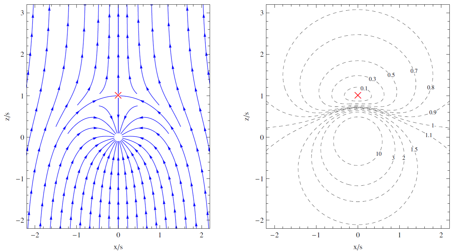
Fig. 1 Wind accretion of an incompressible fluid. The left-hand panel hows the streamlines as described by Equation (22).
The pressure can now be recovered from the Bernoulli constant in Equation (6) as
where we have used the velocity components given in Equations (18) and (19).
From Equation (24) we see that P will become negative at sufficiently small radii. In order to prevent this from happening, we can take the accretor to have a finite radius R and require the central object to fully enclose the region where P < 0. Using Equation (24), it is easy to see that this condition can be satisfied by taking a sufficiently large value for the asymptotic value of the pressure, namely
On the other hand, for fixed asymptotic values v∞ , ρ∞ , P∞ , and a given central accretor of mass M and radius R, this same condition can be rewritten as an upper limit on the accretion rate:
Furthermore, in order for the central accretor to behave as a true sink, it is necessary to require that R < s, i.e. for the stagnation point to lie outside the accretor. From Equation (20), this condition translates as the following lower limit on the accretion rate
Consistency between the two inequalities in Equations (25) and (27) imposes the following relationship between the rest of the model’s parameters
We have thus found that, with this model, we cannot determine a unique accretion rate
for a given central object and asymptotic gas properties. In other words,
where γ is the polytropic index of the equation of state and
We would like to remark here that the standard result from spherical accretion in Equation (29) should be modified when the accretor radius is comparable or larger than the so-called Bondi radius RB= GM/a2 ∞, in which case the maximum accretion is given by
Note that taking the limit v∞ → 0 in Equation (26) leads to
which is the same value for the maximum accretion rate that results by taking the limiting case γ → ∞ (that corresponds to a → ∞) in Equation (30).
Finally, it is interesting to notice that the equation for the streamlines in Equation (22) is independent of both the mass of the central object M and the fluid pressure. In fact, M only affects directly the fluid’s pressure via Equation (24). Moreover, all of the expressions that we have found remain valid even for M = 0 (provided that a massless sink can be conceived in three dimensions). The role played by M > 0 is to contribute to a steeper pressure gradient and to confine the region of negative pressure to a smaller volume than the one arising for a massless sink.
3. Relativistic model
The relativistic solution found by Petrich et al. (1988) (PST) describes a wind accreting onto a rotating black hole (Kerr spacetime) under the conditions of stationarity and irrotational flow. Similarly to the Newtonian case, an irrotational flow in general relativity can be described by a velocity potential Φ such that4
where h=(e+P)/ρc2 is the relativistic enthalpy, e the relativistic internal energy density,5 uμ=dxμ/dt the four-velocity, and gμν the inverse of the spacetime metric. Substituting Equation (32) into the continuity equation (in this case ∇μ(ρuμ) = 0, where ∇μ stands for the covariant derivative) leads to
In general, Equation (33) is a non-linear equation in Φ except in the special case where h ∝ ρ. Specifically, PST considered a stiff equation of state for which P ∝ ρ2 and P = e.6 With this choice, the fluid’s sound speed is constant and equal to the speed of light c everywhere in the fluid.7
In the case of a non-rotating black hole (i.e. Schwarzschild spacetime), PST found the following expression for the velocity potential
where rg = GM/c2 is the gravitational radius and Γ∞ is the Lorentz factor as measured at infinity
Substituting the velocity potential Φ into Equation (32) leads to the velocity field
The special restrictions that arise in general relativity from demanding a regular solution across the black hole’s event horizon (located at 2 rg for a Schwarzschild spacetime) imply that the PST model is characterized by the unique accretion rate
This is an important difference with respect to the Newtonian solution discussed in the previous section where the accretion rate was a free parameter [at most restricted by the inequalities in Equations (26) and (27)].
Let us now define the constant
as a natural extension of the stream length scale s introduced in Equation (20). Using this definition together with Equation (36), we can rewrite the velocity components in Equations (37) and (38) terms of the coordinate time t as
Just as in the Newtonian case, an equation for the streamlines can be obtained by first combining Equations (41) and (42) as (Karas & Mucha 1993)
and then integrating this differential equation to obtain the following expression
where, as before, the integration constant b corresponds to the impact parameter characterizing each individual streamline.
From the velocity components in Equations (41) and (42) we can see that the stagnation point in this case is located at r = rg +(r2 g+σ2)1/2, θ = 0. Completely analogously to the Newtonian case, from Equation (44) we can show that the critical impact parameter bc = 2 σ corresponds to the unique streamline ending up at the stagnation point. By combining Equations (39) and (40) we obtain the following relationship between the stream length scale σ and the wind speed at infinity
from which we can see that even in the limit v∞ → c, the stagnation point reaches a minimum radius of r ≃ 3.2 rg , i.e. it is always located outside the event horizon.
In Figure 2 we show the streamlines and isocontour levels of the velocity field of the PST model for the particular case σ = 3 rg which, from Equation (45), corresponds to a wind speed at infinity of v∞ ≃ 0.44 c. From this figure [and also from Equations (41) and (42)] we can see that, in addition to the stagnation point, the velocity field also vanishes at the event horizon r = 2 rg . This is only a coordinate effect related to the fact that the light cones close onto themselves when described in terms of the coordinate time t, which implies that t is not well suited for describing physical processes close to the event horizon. Indeed, from Equations (36), (37) and (38), we can see that the velocity components dr/dτ and dθ/dτ do not show this behavior.
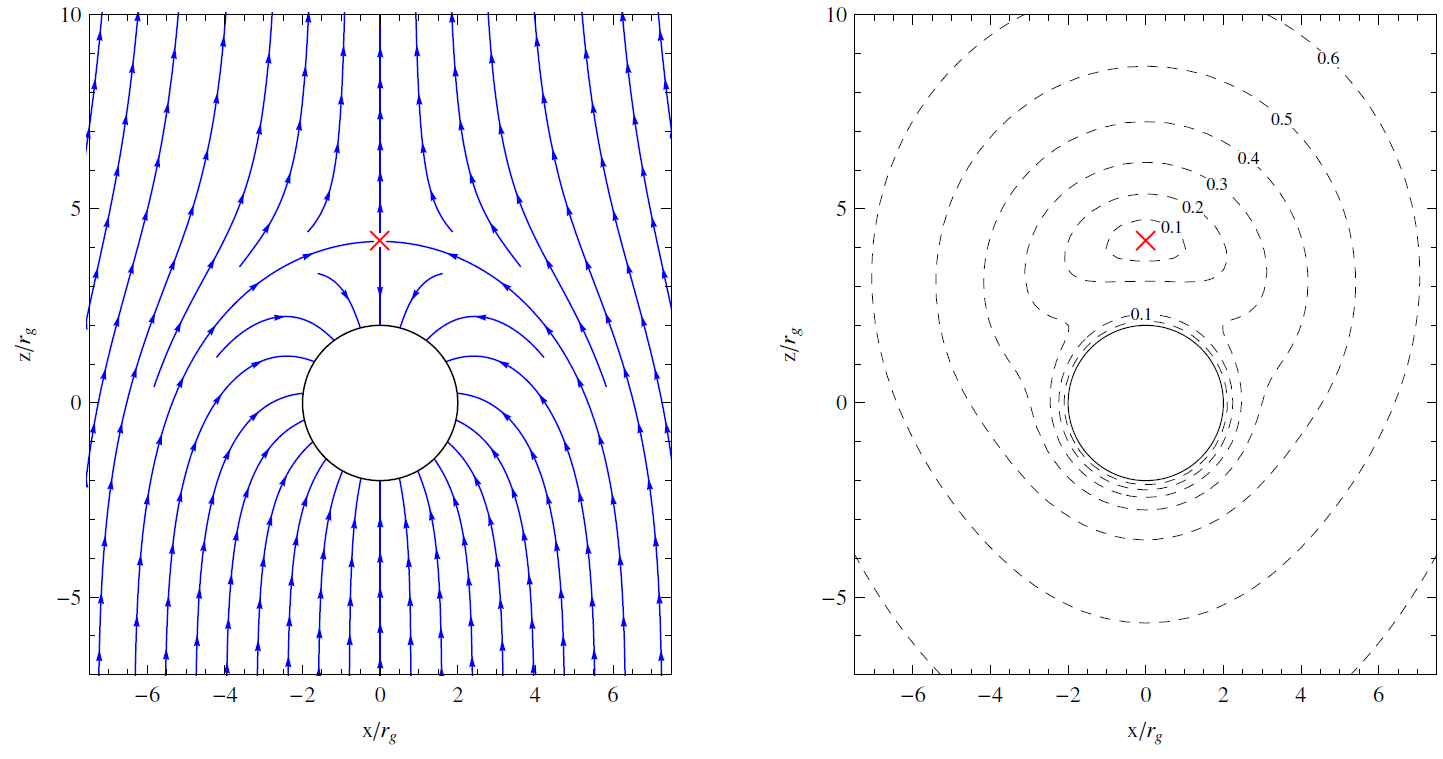
Fig. 2 Wind accretion of the PST model for a Schwarzschild black hole. In this case we have taken σ = 3 rg (which corresponds to v∞ ≃ 0.44 c).
Contrary to the Newtonian model where the resulting flow was described by only one characteristic length scale, namely the stream length scale s, the relativistic model is characterized by two length scales: the stream length scale σ and the gravitational radius rg.
Also in contrast to the Newtonian solution, the rest mass density ρ in the PST model is not constant. An expression for ρ can be found by imposing the normalization condition of the four-velocity (gμνuμuν = −c2) in Equations (36), (37) and (38), which results in
Let us now consider the non-relativistic limit, that is, the regime in which v∞/c≪1 and rg/r≪1. Within this limit, we have that Γ∞ → 1 and σ → s. It then follows that the velocity components in Equations (41) and (42) reduce to the ones corresponding to the Newtonian model in Equations (18) and (19). On the other hand, from the expression for the rest mass density in Equation (46), it follows that ρ → ρ∞ = const. In other words, within the non relativistic limit we recover the incompressible flow approximation on which we based our Newtonian solution.
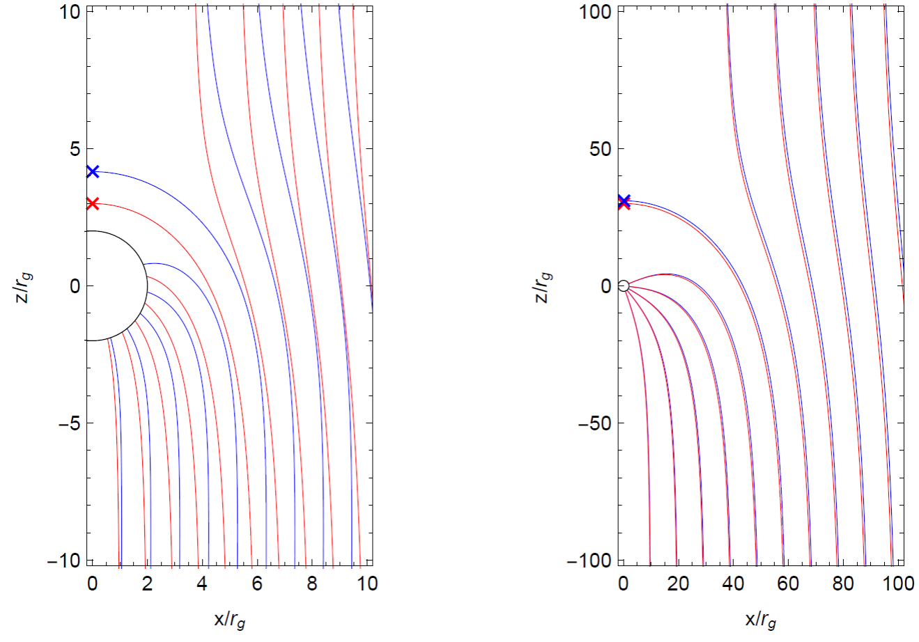
Finally, in order to facilitate the comparison between the Newtonian and the PST models, in Figure 3 we show the corresponding streamlines side by side for two cases: s= σ= 3rg ands=σ=30rg. From Equation (45) it is simple to see that σ ≫ rg implies v∞ ≪ c. Therefore, as the ratio σ/rg grows, the non-relativistic limit should be recovered, just as we can confirm by comparing the left and right panels of this figure.
4. Summary
In this paper, we have presented a simple analytic model of wind accretion for an incompressible fluid falling onto a massive gravitating object. We have shown that this model constitutes a probe into the highly subsonic regime with M ≃ 0. Moreover, this solution corresponds to the Newtonian limit of the relativistic model of wind accretion onto a black hole found by Petrich et al. (1988) (PST). The fluid in the PST model obeys a stiff equation of state P = e for which the sound speed is constant everywhere and equal to the speed of light. In hindsight, it is not surprising that the Newtonian limit of such a fluid corresponds precisely to an incompressible fluid for which the sound speed is, formally, equal to infinity.
The incompressible fluid approximation effectively decouples the flow dynamics from the central object’s gravitational field. This is reflected in the fact that the expression for the streamlines given in Equation (22) is independent of the accretor mass M . Only the fluid’s pressure is directly influenced by M , as expressed in Equation (24). We have found that as M increases, the pressure gradient becomes steeper so as to oppose the enhanced gravitational attraction, and, at the same time, the negative pressure region becomes confined to a smaller volume.
The Newtonian model features only one characteristic length scale: the stream length scale s = (M/4πρ v∞ )1/2. In addition to this the PST model is also characterized by the gravitational radius rg = GM/c2. The existence of these two characteristic length scales leads to a richer variety of flow morphologies than that of the Newtonian model (see Figure 3). The Newtonian model is recovered in the limit s ≫ rg which naturally coincides with the non-relativistic limit v∞ ≪ c.
Another difference between the Newtonian and relativistic models is that, in the former, the accretionrateM isanexternalparameterofthemodel(at most restricted by the inequalities in Equations (26) and (27)) while, in the latter, it has to have the fixed value M= 16π(GM)2ρ∞Γ∞/c3 in order to guarantee a regular solution across the black hole’s event horizon.
The Newtonian model presented in this article can be used as an illustrative example in a gas dynamics course. Moreover, it should be useful as a benchmark for testing Newtonian hydrodynamics codes.

