2.1. Union2.1 SNIa sample

The Union2.1 is one of the largest compilations of supernovae of type la (^{Suzuki et al. 2012}). It originally consisted of 833 SNe drawn from 19 different datasets, but after a variety of homogenization selection criteria (eg. lightcurve quality cuts) 580 remained, out of which there are 546 SNIa with z ≥ 0.02 and 29 with z > 1. The high-redshift SNIa are extremely important to calculate the cosmological parameters, because the differences of various dark energy (DE hereafter) models are larger and more significant at such redshifts (for example see Figure 1 in ^{Plionis et al. 2011}).

Fig. 1 Pie diagram of the 580 SNIa of the Union2.1 set 

We note that the final Union2.1 SNIa distance moduli provided and used in the current paper have been obtained by assuming a common correction for the "stretch", color and host-galaxy parameters for all SNIa (^{Suzuki et al. 2012}), independent of their direction.

In order to visualize the angular and redshift distribution of the Union2.1 SNIa sample, we constructed a pie diagram with the redshift, z, being the radius and the right ascension, α, being the angle (Figure 1). As we can see the higher-z SNIa are detected preferentially along specific directions, some of which contain more data than others. This non-uniform distribution of data, in terms of coordinates, is a result of the fact that the observational campaigns cover very small solid angles of the sky.

2.2. Quantifying the Hubble flow

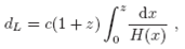
The basic procedure by which the Hubble expansion is traced observationally is through the so-called distance modulus, μ, defined by:

1

where m and M are the apparent and absolute magnitude of the SNIa, and d _L, its luminosity distance, given for a flat geometry (Ωk = 0) by:

2

with H(z) the so-called Hubble parameter defined, using the 1st Friedmann equation, by:

3

with H ₀ the Hubble constant and Ω _m,o, Ω_k,o, Ω_g the fractional densities of matter, curvature and the cosmological constant or DE, respectively, at the present epoch, while w is the equation of state parameter of dark energy. It is evident that the luminosity distance depends strongly on the cosmological parameters. Different DE models modify the functional form of ω(x). The QDE model (Quintessence DE), that we will use in the current study, assumes a constant equation of state parameter, ω, which can admit values different from -1.

The assumption of an isotropic Hubble expansion implies a Hubble parameter H(z) being a function only of z and not of direction. Therefore, different radial directions should provide statistically equivalent H(z). The approach we use in this analysis is to investigate different radial directions, or solid angles, in order to confirm or not the independence of H(z) on direction. The criterion of equivalence of the Hubble expansion for different solid angles will be whether the resulting cosmological parameters, (Ω _m o,ω), provided by fitting the data to the Hubble expansion models, are statistically consistent among themselves and with the solution using the whole (z > 0.02) Union2.1 compilation.

2.3. The X ² - minimization procedure

In order to fit the cosmological parameters of equation (3) we minimize the difference between the SNIa observed distance moduli and the theoretical ones via equation (1). To this end we use a X ² minimization procedure outlined below.

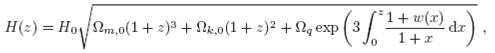
Suppose we have a measurement of the distance modulus μ _0bs(z_i) with an uncertainty σμ, which arises from its redshift z _i . The theoretically expected distance modulus for the same redshift z _i is μ, _th(z_i, p), with p ≡ ω,Ω _m0 being the model's free parameters. Now suppose that we have N μ _0bs (z_i ) independent measure ments. The total probability of obtaining this entire set of N data points is equal to the product of the probability for each data point, so :

4

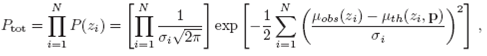
If we want to find the maximum probability we have to minimize the sum in the exponential term of P_tot, and therefore, this quantity is defined as:

5

the minimum value of which, X ² _min, provides the maximum probability of P_tot. Thus, since the theoretical expected μ _th (z_i,p), depend on a set of free parameters, which correspond to the elements of the vector p [ in our case p = (Ω _m o,ω) ], we can test for which values of these parameters we obtain the maximum probability. In our analysis we ignore the covariance matrix of the errors in the observed SNIa distance moduli and use the root-mean-square of the diagonal elements, provided by the Union2.1 catalogue. In addition, we use the approach of ^{Nesseris & Perivolaropoulos (2006)} with which we do not need to impose an a priori value of the Hubble constant.

The best fit value of the free parameters, po, is provided by the X ² _min. When the parameters differ from these values, p ≠ po, then the X ² increases, so ∆x ² = X ² - X ² _min > 0. Limits of ∆x ² that depend on the number of the fitted parameters N _f , define confidence regions that contain a certain fraction of the probability distribution of p's. For our case of N _f = 2, the 1, 2 and 3 σ confidence regions correspond to ∆x ² = 2.3, 6.17 and 11.83, respectively.

3.1. Dividing the sky into nine solid angles

As a first test, we divided the celestial sphere into nine fully independent solid angles, as shown in Figure 2, so that each one has a similar number of SNIa. We then fitted the QDE cosmological parameters in each zone, by using the previously described minimization procedure. We identified one sky region with a distinctly different Ω _m,o -ω solution as compared with other regions of the sky, as well as with the whole Union2.1 sample. This region, which we call Group X, contains 82 SNIa and has galactic coordinates within: 35° < l < 83° and -79° < b < -37° (the red region in Figure 2). We have verified that the SNIa redshift distribution in this region does not present any "peculiarity" with respect to the overall distribution. In fact, although the redshift distributions of the separate regions show inconsistencies with the overall Union2.1 redshift distribution (with corresponding Kolmogorov-Smirnov probabilities varying from Ƥ ≃ 10^-7 up to ~ 0.13), that of Group X is the most statistically consistent with the overall distribution (Ƥ ≃ 0.13). Thus a "peculiar" redshift distribution is not the cause of the behavior of the (Ω_m,o - ω ) solution for Group X.

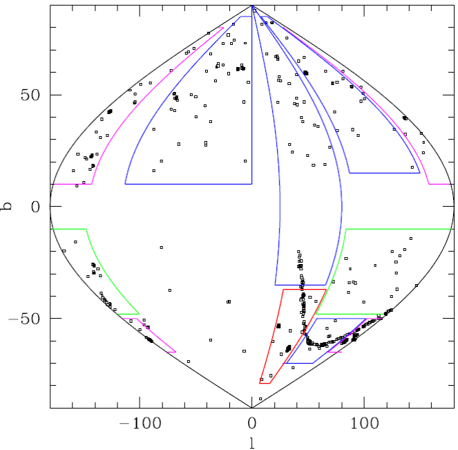
Fig. 2 The celestial sphere in equal area projection with 8 separate regions delineated (the 9th region is the rest of the sky). The red area corresponds to Group-X. Magenta and green colours are used when a region folds over into the Galactic longitude direction. The color figure can be viewed online. 

In the left panel of Figure 3 we compare the 1σ contour region of Group X with that of the rest of the Union2.1 sample. It is clear that their respective 1σ contour regions have no common area, indicating a relatively significant difference. Quantitatively, the difference of the latter best-fit solution with respect to that of Group X is ∆x ² ≃ 4.3 (i.e., the probability of their being different is ≃ 90%).

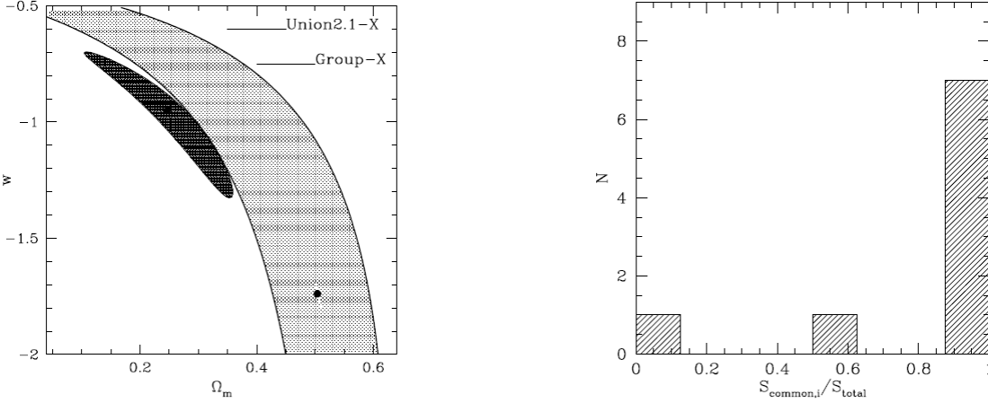
Fig. 3 Left panel: 1σ contour plots of Group X (dark gray contour, 82 SNIa) and for the rest of the Union2.1 data (light gray contour, 464 SNIa). Right panel: Distribution of the common 1σ contour area (between each of the 9 individual subsamples and the whole SNIa sample) divided by the 1σ area of the entire sample. 

In order to visualise the uniqueness of the behaviour of Group X we plot in the right panel of Figure 3 the fraction of the QDE 1σ contour area, based on the whole Union2.1 (excluding the Group X), which is common with that based on every one of the 9 independent subsamples of SNIa. We observe that the 1σ solution space of the entire sample is fully (100%) encompassed within almost each one of the other 8 subsamples (with one exception, which is at 60% and is shown in green in Figure 2). Remarkably, Group X is at 0%.

It is interesting to note that Group X is located close to the CMB dipole anti-apex direction. Furthermore, many studies have consistently found the largest deviations from an isotropic expansion occurring near this direction. For example, as early as 2001 and using only 79 SNIa, ^{Kolatt & Lahav (2001)} found a Hubble diagram dipole pointing towards (l,b) ≃ (80°,-20°). ^{Antoniou & Perivolaropoulos (2010)} using the Union2 SNIa sample and, separately, ^{Cooke & Lynden-Bell (2010)}, using the slightly earlier Union sample, also found a preferred axis of minimum acceleration in the same general direction, although at a low significance level.

Yang, Wang & Chu (2013) using the Union2.1 SNIa data also found a low significance preferred direction of the accelerating expansion. Finally, ^{Javanmardi et al. (2015)}, found as the most discrepant direction of the Hubble expansion the region centered on (l, b) ≃ (67.5°, -66.4°), which indeed coincides with our Group X.

3.2. Possible systematic effects

The statistically important "erratic" behaviour of Group X with respect to the rest of the SNIa could be due to a variety of reasons, among which are: an intrinsic anisotropy of the Hubble expansion, a large bulk flow in this part of the sky or some unknown systematic observational error (see for example ^{Heneka et al. 2014}). In this respect we remind the reader that the SNIa distance moduli, provided in the Union2.1 compilation, have been derived assuming a global correction for individual deviations from the average SNIa light-curve and from the mean color. As highlighted in ^{Javanmardi et al. (2015)}, the most robust approach for testing isotropy would be to find the values for the "stretch", color and host-galaxy parameters for each patch of the sky separately. However, we adopt the simplified approach of the global correction, as in ^{Javanmardi et al. (2015)}.

Below we present our analysis of two possible systematic observational effects that could be the cause of the "erratic" behaviour of Group X.

3.2.1. Galactic absorption

We tested whether the erratic behaviour of Group X could be due to an inadequate treatment of the Galactic absorption. To this end, we plotted for each SNIa (left panel of Figure 4) the distance modulus deviation from that expected in the concordance model, ie., ∆μ = μ _obs (z_i ) -μ _th (z_i,p) with p ≡ (ω,Ω_{m, o}) ≡ ( - 1.013,0.282), as a function of the Galactic latitude |b|.

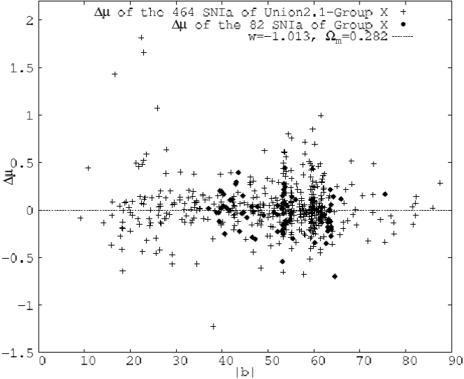
Fig. 4 Distance moduli deviation ∆μ, with respect to that of (Ω _m , _o,ω ) = (0.282,-1.013), as a function of galactic latitude |b| for the 546 Union2.1 SNIa (crosses) and for the 82 SNIa of Group X (large dots). 

As illustrated in Figure 4, the SNIa distance moduli of Group X (large dots) do not show a distinct behaviour as a function of |b|. However, we see that the SNIa with the largest ∆μ's, i.e., the apparently faintest ones, are all at small |b|'s, which strongly hints towards at least some SNIa having magnitudes inadequately corrected, or overcorrected, for Galactic absorption. These SNIa (1997k with b = 16.6°, 19971 with b = 22.4° and 1997o with b = 22.9°) are also among the closest to the plane of the Galaxy.

3.2.2. SNIa Outliers ?

We have investigated the possibility of whether an erratic behaviour of one or a few SNIa could cause the mentioned effect. To this end we systematically excluded, one by one, each of the SNIa of Group X and checked whether the QDE 1σ contour area of the remaining Group X increased its consistency with the Union2.1 solution (excluding the Group X). We found that, although the large majority of the single SNIa do not have any major contribution to the erratic behaviour of Group X, some individual SNIa do have a very large effect on the Group X solution, as can be seen in Figure 5 where we plot the fraction of the overall Union2.1 (excluding the Group X) 1σ contour area covered by the corresponding Group X 1σ contour area when excluding one SNIa at a time. The three cases that show a > 20% effect are shown in black. The largest effect, that of a ≈ 35% recovery of the common 1σ solution space, is due to excluding the 03D4.cx SNIa at z = 0.949. The next most important effect is due to g050 at z = 0.613. By excluding it we obtain a ≈ 25% recovery of the common 1σ solution space, while the third most important effect, again at a ≈ 23% level, is due to the 2005hv at z = 0.1776. Most importantly, the joint effect of excluding all three "erratic" SNIa is the increase of the consistency from 0% to more than 93%, thus annulling the tension between the Group X and the rest of the Union2.1 sample solution.

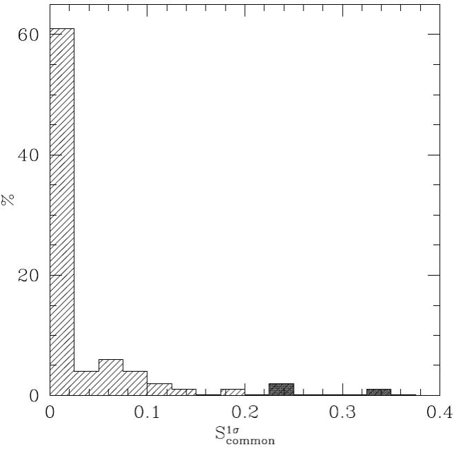
Fig. 5 Fraction of the Union2.1 (excluding Group X) QDE 1σ solution area which is common with the corresponding area of Group X excluding one by one each Group X SNIa from the fitting procedure. Marked by dark shade are the three SNIa with the largest effect, the exclusion of which recovers the consistency of the Hubble expansion of Group X with that of the overall Union2.1 sample. 

We conclude that the identified inconsistency of the Hubble expansion of the SNIa of Group X appears to be dominated by the erratic behaviour of only three out of the 82 SNIa, highlighting the sensitivity of the Hubble expansion solution to outliers when small numbers of SNIa are investigated.

Excluding from the overall analysis the above three "erratic" SNIa, as well as the three SNIa at low galactic latitudes, which may be inadequately corrected for Galactic absorption, we find:

7

with X ²/dof = 0.909. Comparing this result with the solution using all the Union2.1 set (equation 6) we see a small but perceptible difference of the best fit Ω _m,o,ω parameter values, while the X ²/dof is also smaller.

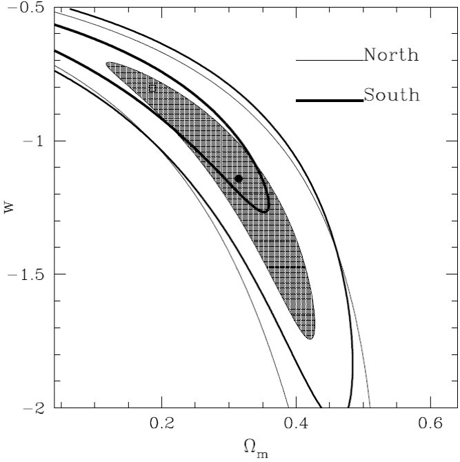
3.3. Separate Galactic hemispheres solutions

We now consider, as a final test of possible Hubble expansion anisotropies, the southern and northern Galactic hemispheres separately, excluding the 6 "erratic" SNIa previously identified. We therefore use 332 and 208 SNIa, respectively for the southern and northern hemispheres. The results are:

South : ω = -0.805 ± 0.084, Ω _m,0 = 0.186-0.0468+0.0508 X ² _min/dof = 0.9492

North: ω = -1.144-0.1440)+0.1325 , Ω _m,0 = 0.315-0.0377+0.0405 X ² _min/dof = 0.8500

It can be seen that the best-fit QDE model parameters for the two hemispheres are quite different, with a ∆x ² = 1.27, but within the 1σ uncertainty contour range, as shown in Figure 6. Therefore this difference indicates some tension between the two hemisphere solutions, but does not appear to constitute evidence of a significant anisotropy.

Fig. 6 The separate Galactic hemisphere solution: Thick line contours corresponds to the Southern G.H. and gray scale and thin lines to the Northern G.H. with their best fit values shown as empty and filled dots, respectively.