SciELO - Scientific Electronic Library Online

 
vol.68 número5The effect of sound vibration towards the stomata pore area via edge detection analysis índice de autoresíndice de materiabúsqueda de artículos
Home Pagelista alfabética de revistas  

Servicios Personalizados

Revista

Articulo

Indicadores

Links relacionados

  • No hay artículos similaresSimilares en SciELO

Compartir


Revista mexicana de física

versión impresa ISSN 0035-001X

Rev. mex. fis. vol.68 no.5 México sep./oct. 2022  Epub 17-Feb-2023

https://doi.org/10.31349/revmexfis.68.051403 

Research

Other areas in Physics

On some novel solitons solutions to the generalized (3 + 1)-dimensional Boiti-Leon-Manna-Pempinelli model using two different approaches

K. U. Tariqa 

M. Incb  c  d  * 

R. Javeda 

a Department of Mathematics, Mirpur University of Science and Technology, Mirpur-10250 (AJK), Pakistan.

b Department of Computer Engineering, Biruni University, 34025 Istanbul, Turkey.

c Science Faculty, Department of Mathematics, Firat University, 23119 Elazig, Turkey.

d Department of Medical Research, China Medical University Hospital, China Medical University, Taichung, Taiwan.


Abstract

In this study we investigate Boiti-Leon-Manna-Pempinelli equation in three dimensions, which describes the evolution of the horizontal velocity component of water waves propagating in the xy-plane in an infinite narrow channel of constant depth and that can be considered as a model for incompressible fluid. The new (F/G)-expansion approach and the unified approach are employed to construct some new traveling wave solutions to the nonlinear model. A large numbers of traveling wave solutions for the nonlinear model are demonstrated respectively in the form of hyperbolic and trigonometric function solutions. The proposed methods are also proved to be effective in solving nonlinear evolution problems in mathematical physics and engineering.

Keywords: New (F/G)-expansion method; the unified method; traveling waves solutions; nonlinear evolution equations; exact solutions

1. Introduction

The nonlinear partial differential equations (NPDEs) are of key importance due to their significant role in diverse disciplines of science and technology, including heat transfer, wave propagation, elasticity, fibres, condensed matter physics, fluid dynamics, hydrodynamics, and nuclear physics. The nonlinear wave structures have fascinated many researchers in the recent decades due to their numerous properties observed in numerous disciplines. In the presence of solitary waves, the nonlinear evolution models are utilized to simulate the effect of surface for deep water and weakly nonlinear dispersive long waves. Therefore, the exact solutions of such models play a vital role to study the dynamical behaviour and further properties of physical phenomenon occurring in several fields such as electromagnetism, physical chemistry, geophysics, ionised physics, elastic medium, fluid motion, fluid mechanics, elastic medium, nuclear physics, electrochemistry, optical fibres, energy physics, chemical mechanics, gravity, biostatistics, statistical and natural physics [1-7].

To investigate the behaviour of ultra-modern models, renowned researchers from all over the world are able to devise a variety of interesting numerical and analytical approaches. As a result, the study of nonlinear wave structures has latterly received a lot of attention. The Tanhcoth expansion function technique [8, 9], the sub ODE method [10, 11], the sine-Gordon technique [12-14], the first integral technique [15-17], the modified Kudryashov approach [18], the extended simplest equation method [19-21], the modified simple equation method [22-24], the Kudryashov-expansion method [25], the Lie symmetry technique [26, 27], the extended Tanh technique [28, 29], the modified Khater method [30], and the Homogeneous balance method [31, 32], are some of the key approaches which have been found in current decades.

The (3+1)-dimensional Boiti-Leon-Manna-Pempinelli (BLMP) model is an extension of the 2-dimensional BLMP model that describes the three dimensional interconnection of the Riemann travelling wave solutions along x and y-axis [33, 34], which reads

-3uxuxy+uxz-3uxxuy+uz+uxxxy+uxxxz+uyt+uzt=0, (1)

where u is a function which depends on the coordinates (x, y, z, t). Darvishi et al. studied the one wave and different numerous waves solutions for the three dimensional BLMP problem by employing different exp-function approaches [35]. Xu developed four types of lump solutions using the Painleve-Backlund transformation [36, 37], with two N exponential functions and quadratic functions. The multi-ple exponential function approaches [38, 39] and scale trans-formation approaches [40, 41] were also used to investigate the BLMP equation by Tang and Zai. Ma et al., being used to calculate the precise three-wave solutions. Exact solutions, such as periodic wave solutions, periodic solitary waves, and kink solutions can be found. Using Hirotas bilinear approach, were also generated three soliton waves results in words of kink periodic wave solutions. By employing the group trans-formation approach [42, 43], Mabrouk et al. are able to develop various appealing analytical solutions.

The basic aim of this study is to use two efficient approaches to get traveling and solitary waves solutions to the (3+1)-BLMP model namely the (F/G)-expansion technique [44] and unified technique [45, 46]. The aforementioned approaches are traveling wave solutions that can be expressed by a polynomial in (F/G) and Θ (X). Traveling and the solitary waves solutions to the dynamical model are examined physically and analytically.

2. Description of proposed methods

2.1. The new (F/G)-expansion method

Consider the NPDE in the following form

Fϕ,ϕt,ϕx,ϕtt,ϕxx,ϕxt,=0, (2)

φ is an unknown function of the variables x and t and F is a polynomial in φ(x,t) and its partial derivatives, involving highest derivatives and nonlinear terms. Suppose the following transformation

ϕ(x,t)=ϕ(η), η=x-ct, (3)

where c is a non-zero constant. The travelling wave variable η allows us to reduce Eq. (2) to an ODE for φ = φ(η)

Qϕ,ϕ',ϕ'',ϕ''',=0. (4)

The major process of new F/G-expansion method is outlined below:

Step 1. The solution of Eq. (4) will be in (F/G) as follows,

ϕ(η)=i=0naiFGi, (5)

where G = G(η) and F = F(η) satisfy

F'(η)=λG(η),G'(η)=μF(η), (6)

a 0, a 1, · · · , a m , λ and µ are constants to be calculated later, a m ≠ 0.

Step 2. Furthermore, N is a positive integer that can be calculated by using the homogeneous balance principle between the higher derivatives and nonlinear terms in ODE Eq.(4). We may get the following solutions of F(η) and G(η), with the help of Eq.(6), which are listed as below,

Case I. If λ > 0, μ > 0, we get the hyperbolic function solution

F(η)=C2λsinhλμημ+C1coshλμη,G(η)=C1μsinhλμηλ+C2coshλμη. (7)

Case II. If λ < 0, µ < 0, we get the hyperbolic function solution

F(η)=C1cosh-λ-μη-C2-λsinh-λ-μη-μ,G(η)=C2cosh-λ-μη-C1-μsinh-λ-μη-λ. (8)

Case III. If λ > 0, µ < 0, we get the trigonometric function solution

F(η)=C2λsinλ-μη-μ+C1cosλ-μη,G(η)=C2cosλ-μη-C1-μsinλ-μηλ. (9)

Case IV. If λ < 0, µ > 0, we get the trigonometric function solution

F(η)=C1cos-λμη-C2-λsin-λμημ,G(η)=C1μsin-λμη-λ+C2cos-λμη. (10)

Step 3. Putting Eq. (5) and Eq. (6) into Eq. (4) a group of algebraic equations for(F/G) i (i = 1, 2, . . . , m) is obtained. Setting all (F/G) i to zero and solving these nonlinear algebraic equations we get different accurate solutions of Eq. (2) according to (3), (5), (7), (8) and (9), (10).

2.2 The unified method

The major process of unified method is outlined below,

Step 1. The solution of Eq. (4) is then assumed and may be written as follows,

u(X)=A0+i=1NAiΘi(X)+BiΘ-i(X), (11)

where A i , B i (i = 0, 1, ......, N) are constants to be determined, N is a possitive integer and Θ(X) satisfies the Riccati differential equation,

Θ'(X)=γ+Θ2(X), (12)

where Θ’ = dΘ/dX and γ is a real constant. Equation (12) has the following exact solutions.

Family 1. If γ < 0, then

Θ(X)=±γ-A2+B2-A-γcosh2-γη0+XAsinh2-γη0+X+B,Θ(X)=±-γ+A-γ(2)A+cosh2-γη0+Xsinh2-γη0+X. (13)

Family 2. If γ > 0, then

Θ(X)=±γA2-B2-Aγcos2γη0+XAsin2γη0+X+B,Θ(X)=±iγ+Aiγ(2)A+cos2γη0+XiSin2γη0+X. (14)

Family 3. If γ = 0, then

Θ(X)=-1η0+X, (15)

where A, B and η 0 are real arbitrary constants.

Step 2. The positive integer N in Eq. (11) can be determined by homogeneous balance principle between the higher derivatives and nonlinear terms in ODE Eq. (4).

Step 3. Putting Eq. (11) along with Eq. (12) into Eq. (4) and setting the coefficients of Θ i (i = 0, ±1, ±2, ...) to zero, we get the system of equations.

Step 4. After solving the system of algebraic equations, we substitute the obtained constants together with the solution of Eq. (12) into Eq. (11) to obtain exact solutions of Eq. (2).

3. Soliton structures

3.1 Application to the new (F/G)-expansion approach

Consider the wave transformation

ux,y,z,t=ψX, with

X=νt+κx+μy+λz, (16)

where λ, µ, ν and κ are constants. Substituting values from Eq. (16) to Eq. (1). We obtain the following ordinary differential equation,

κ3ψ(4)-6κ2ψ'ψ''+νψ''=0. (17)

By using the homogeneous balance principle we obtain N = 1.

The solution of Eq. (17) has the form

ψ(X)=a0+a1F(X)G(X). (18)

Putting Eq. (18) into Eq. (17), collecting all same powers terms of (F/G) together, and setting each (F/G) polynomial to zero yields the following group of algebraic system of equations

16a1κ3λ2μ2+12a12κ2λ2μ-2a1λμν=0, -40a1κ3λμ3-24a12κ2λμ2+2a1μ2ν=0,24a1κ3μ4+12a12κ2μ3=0.

Solving the above algebraic problem results in the values

a1=23μ2/3ν3λ3, κ=-ν322/3λ3μ3.

Substituting the above results into Eq. (18), produces the following four categories of traveling wave solutions.

Family I.

Case I. When λ > 0, µ > 0, we get the hyperbolic function solution

u1(x,y,z,t)=a0+23μ2/3ν3C2λsinhλμXμ+C1coshλμXλ3C1μsinhλμXλ+C2coshλμX, (19)

where X = νt + κx + µy + λz, C 1 and C 2 are arbitrary constants. If C 1 = 0, then we obtain the solitary wave solution

u1(x,y,z,t)=a0+23λ6μ6ν3tanhλμX. (20)

Case II. When λ < 0, µ < 0, we get the hyperbolic function solution

u2(x,y,z,t)=a0+23μ2/3ν3ζλ3(C2cosh(-λ-μX)-η, (21)

where

ζ=C1cosh(-λ-μX)-C2-λsinh(-λ-μX)-μ,

η=C1-μsinh(-λ-μX)-λ,

And X = νt + κx + µy + λz, C 1 and C 2 are arbitrary constants. If C 1 = 0, then we obtain the solitary wave solution

u2(x,y,z,t)=a0-23-λμ2/3ν3tanh-λ-μXλ3-μ. (22)

Case III. When λ > 0, µ < 0, we get the trigonometric function solution

u3(x,y,z,t)=a0+23μ2/3ν3ζλ3C2cosλ-μX-C1-μsinλ-μXλ, (23)

where

ζ=C2λsinλ-μX-μ+C1cosλ-μX,

and X = νt + κx + µy + λz, C 1 and C 2 are arbitrary constants. If C 1 = 0, then we obtain the solitary wave solution

u3(x,y,z,t)=a0+23λ6μ2/3ν3tanλ-μX-μ. (24)

Case IV. When λ < 0, µ > 0, we get the trigonometric function solution

u4(x,y,z,t)=a0+23μ2/3ν3ζλ3C1μsin-λμX-λ+C2cos-λμX, (25)

where

ζ=C1cos-λμX-C2-λsin-λμXμ,

and X = νt + κx + µy + λz, C 1 and C 2 are arbitrary constants. If C 1 = 0, then we obtain the solitary wave solution

u4(x,y,z,t)=a0-23-λμ6ν3tan-λμXλ3. (26)

Family II

a1=--23μ2/3ν3λ3,κ=-13ν322/3λ3μ3.

Substituting the above results into Eq. (18), produces the following four categories of traveling wave solutions.

Case I. When λ > 0, µ > 0, we get the hyperbolic function solution

u5(x,y,z,t)=a0--23μ2/3ν3ζλ3η+C2coshλμX, (27)

where

ζ=C2λsinhλμXμ+C1coshλμX

η=C1μsinhλμXλ

and X = νt + κx + µy + λz, C 1 and C 2 are arbitrary constants. If C 1 = 0, then we obtain the solitary wave solution.

u5(x,y,z,t)=a0--23λ6μ6ν3tanhλμX. (28)

Case II. When λ < 0, µ < 0, we get the hyperbolic function solution

u6(x,y,z,t)=a0--23μ2/3ν3ζλ3C2cosh-λ-μX-η, (29)

where

ζ=C1cosh-λ-μX-C2-λsinh-λ-μX-μ,

η=C1-μsinh-λ-μX-λ,

And X = νt + κx + µy + λz, C 1 and C 2 are arbitrary constants.

If C 1 = 0, then we obtain the solitary wave solution

u6(x,y,z,t)=a0+-23-λμ2/3ν3tanh-λ-μXλ3-μ. (30)

Case III. When λ > 0, µ < 0,we get the trigonometric function solution

u7(x,y,z,t)=a0--23μ2/3ν3(C2λsin(λ-μX)-μ+C1cos(λ-μX)λ3(C2cos(λ-μX)-C1-μsin(λ-μX)λ), (31)

where X = νt + κx + µy + λz, C 1 and C 2 are arbitrary constants. If C 1 = 0, then we obtain the solitary wave solution

u7(x,y,z,t)=a0--23λ6μ2/3ν3tanλ-μX-μ. (32)

Case IV. When λ < 0, µ > 0, we get the trigonometric function solution

u8(x,y,z,t)=a0--23μ2/3ν3(C1cos(-λμX)-C2-λsin(-λμX)μ)λ3(C1μsin(-λμX)-λ+C2cos(-λμX)), (33)

where X = νt + κx + µy + λz, C 1 and C 2 are arbitrary constants.

If C 1 = 0, then we obtain the solitary wave solution

u8(x,y,z,t)=a0+-23-λμ6ν3tan-λμXλ3. (34)

Family III.

a1=(-1)2/323μ2/3ν3λ3,κ=-(-1)2/3ν322/3λ3μ3.

Substituting the above results into Eq. (18), produces the following four categories of traveling wave solutions.

Case I. When λ > 0, µ > 0, we get the hyperbolic function solution.

u9(x,y,z,t)=a0+(-1)2/323μ2/3ν3ζλ3C1μsinh(λμX)λ+C2cosh(λμX), (35)

where

ζ=C2λsinh(λμX)μ+C1cosh(λμX),

and X = νt + κx + µy + λz, C 1 and C 2 are arbitrary constants.

If C 1 = 0, then we obtain the solitary wave solution

u9(x,y,z,t)=a0+(-1)2/323λ6μ6ν3tanhλμX. (36)

Case II. When λ < 0, µ < 0, we get the hyperbolic function solution.

u10(x,y,z,t)=a0+(-1)2/323μ2/3ν3ζλ3(C2cosh(-λ-μX)-C1-μ(sinh(-λ-μX-λ), (37)

where

ζ=C1cosh-λ-μX-C2-λsinh-λ-μX-μ,

and X = νt + κx + µy + λz, C 1 and C 2 are arbitrary constants.

If C 1 = 0, then we obtain the solitary wave solution

u10(x,y,z,t)=a0-(-1)2/323-λμ2/3ν3tanh-λ-μXλ3-μ. (38)

Case III. When λ > 0, µ < 0, we get the trignomatric function solution

u11(x,y,z,t)=a0+(-1)2/323μ2/3ν3ζλ3(C2cos(λ-μX)-C1-μsin(λ-μX)λ), (39)

where

ζ=C2λsin(λ-μX)-μ+C1cos(λ-μX

and X = νt + κx + µy + λz, C 1 and C 2 are arbitrary constants.

If C 1 = 0, then we obtain the solitary wave solution

u11(x,y,z,t)=a0+(-1)2/323λ6μ2/3ν3tanλ-μX-μ. (40)

Case IV. When λ < 0, µ > 0, we get the trignomatric function solution

u12(x,y,z,t)=a0+(-1)2/323μ2/3ν3ζλ3C1μsin(-λμX)-λ+C2cos(-λμX), (41)

where

ζ=C1cos(-λμX)-C2-λsin(-λμX)μ,

and X = νt + κx + µy + λz, C 1 and C 2 are arbitrary constants.

If C 1 = 0, then we get the solitary wave solution

u12(x,y,z,t)=a0-(-1)2/323-λμ6ν3tan(-λμX)λ3. (42)

4. Application to the unified method

By using the homogeneous balance principle we obtain N=1. Thus the solution of Eq. (17), is

u(X)=A0+A1Θ(X)+B1Θ-1(X). (43)

Putting Eq. (43) into Eq. (17), collecting all same powers terms of Θ i together and setting the coefficients of Θ i (i = 0, ±1, ±2, ...) to zero, we get the system of equations

24B1γ4κ3+12B12γ3κ2=0,-12A1B1γ3κ2+40B1γ3κ3+24B12γ2κ2+2B1γ2ν=0,-12A1B1γ2κ2+16B1γ2κ3+12B12γκ2+2B1γν=0,12A1B1γκ2+16A1γ2κ3-12A12γ2κ2+2A1γν=0,12A1B1κ2+40A1γκ3-24A12γκ2+2A1ν=0,24A1κ3-12A12κ2=0.

Solving the above algebraic problem, the following are the outcomes:

Family I.

A1=--123ν3γ3,  B1=-123γ23ν3,   κ=--123ν32γ3.

Putting above results into Eq. (43), produces following categories of traveling wave solutions.

Case I. When γ < 0, we get the solution

u13(x,y,z,t)=A0--123ν3ζγ3Asinh2-γη0+X+B+-123γ2/3ν3Asinh2-γη0+X+Bζ, (44)

where

ζ=±γ-A2-B2-A-γcosh2-γη0+X.u14(x,y,z,t)=A0--123ν3ζγ3+-123γ2/3ν3ζ, (45)

where

ζ=A-γ(2)A+cosh2-γη0+Xsinh2-γη0+X±-γ,

and X=νt-(-1/23ν3x/2γ3)+μy+λz, and A, B and η 0 are real arbitrary constants.

Case II. When γ > 0, we get the solution

u15(x,y,z,t)=A0--123ν3ζγ3Asin2γη0+X+B+-123γ2/3ν3Asin2γη0+X+Bζ, (46)

where

ζ=±γA2-B2-Aγcos2γη0+X.u16x,y,z,t=A0--123ν3ζγ3+-123γ2/3ν3ζ, (47)

where

ζ=Aiγ(2)A+cos2γη0+XiSin2γη0+X+γ±i,

X=νt-(-1/23ν3x/2γ3)+μy+λz, and A, B and η 0 are real arbitrary constants.

Case III. When γ = 0, then we get the solution.

u17(x,y,z,t)=A0+-123γ2/3ν3-η0-X+-123ν3γ3η0+X, (48)

where X=νt-(-1/23ν3x/2γ3)+μy+λz, and η 0 is a real arbitrary constant.

Family II.

B1=0,κ=ν322/3γ3,A1=23ν3γ3.

Putting the above results into Eq. (43), produces following four categories of traveling wave solutions.

Case I. When γ < 0, we get the solution

u18(x,y,z,t)=A0+23ν3ζγ3Asinh2-γη0+X+B, (49)

where

ζ=±γ-A2-B2-A-γcosh2-γη0+X.u19(x,y,z,t)=A0+23ν3ζγ3, (50)

where

ζ=A-γ(2)A+cosh2-γη0+Xsinh2-γη0+X±-γ,

X=νt+(ν3x/22/3γ3)+μy+λz, and A, B and η 0 are real arbitrary constants.

Case II. When γ > 0, we get the solution

u20(x,y,z,t)=A0+23ν3±γA2-B2-Aγcos2γη0+Xγ3Asin2γη0+X+B, (51)

u21(x,y,z,t)=A0+23ν3ζγ3, (52)

where

ζ=Aiγ(2)A+cos2γη0+XiSin2γη0+X+γ±i,

X=η0+νt+(ν3x/22/3γ3)+μy+λz, and A, B and η 0 are real arbitrary constants.

Case III. When γ = 0, then we get the solution

u22(x,y,z,t)=A0-23ν3γ3η0+X, (53)

where X=η0+νt+(ν3x/22/3γ3)+μy+λz, and η 0 is a real arbitrary constant.

Family III.

κ=ν3223γ3,A1=ν323γ3,B1=-γ2/3ν323.

Putting the above results into Eq. (43), produces following four categories of traveling wave solutions.

Case I. When γ < 0, we get the solution

u23(x,y,z,t)=A0-γ2/3ν3Asinh2-γη0+X+B23ζ+ν3ζ23γ3Asinh2-γη0+X+B, (54)

where

ζ=±γ-A2-B2-A-γcosh2-γη0+X,u24(x,y,z,t)=A0-γ2/3ν323ζ+ν3ζ23γ3, (55)

where

ζ=A-γ(2)A+cosh2-γη0+Xsinh2-γη0+X±-γ,

X=η0+νt+(ν3x/223γ3)+μy+λz and A, B and η 0 are real arbitrary constants.

Case II. When γ > 0, we get the solution

u25(x,y,z,t)=A0-γ2/3ν3Asin2γη0+X+B23ζ+ν3ζ23γ3Asin2γη0+X+B, (56)

where

ζ=±γA2-B2-Aγcos2γη0+X.u26(x,y,z,t)=A0-γ2/3ν323ζ+ν3ζ23γ3, (57)

where

ζ=Aiγ(2)A+cos2γη0+XiSin2γη0+X+γ±i,

X=η0+νt+(ν3x/223γ3)+μy+λz, and A, B and η 0 are real arbitrary constants.

Case III. When γ = 0, then we get the solution

u27(x,y,z,t)=A0-γ2/3ν3-η0-X23-ν323γ3η0+X, (58)

where X=η0+νt+(ν3x/223γ3)+μy+λz, and η 0 is a real arbitrary constant.

Family IV.

A1=0,κ=(-1)2/3ν322/3γ3),B1=-(-1)2/323γ2/3ν3.

Putting the above results into Eq. (43), produces following four categories of traveling wave solutions.

Case I. When γ < 0, we get the solution

u28(x,y,z,t)=A0-(-1)2/323γ2/3ν3Asinh2-γη0+X+B±γ-A2-B2-A-γcosh2-γη0+X, (59)

u29(x,y,z,t)=A0-(-1)2/323γ2/3ν3A-γ(2)A+cosh2-γη0+Xsinh2-γη0+X+±-γ, (60)

where X=νt+((-1)2/3ν3x/22/3γ3)+μy+λz and A, B and η 0 are real arbitrary constants.

Case II. When γ > 0, we get the solution

u30(x,y,z,t)=A0-(-1)2/323γ2/3ν3Asin2γη0+X+B±γA2-B2-Aγcos2γη0+X, (61)

u31(x,y,z,t)=A0-(-1)2/323γ2/3ν3Aiγ(2)A+cos2γη0+XiSin2γη0+X+γ±i, (62)

where X=νt+((-1)2/3ν3x/22/3γ3)+μy+λz, and A, B and η 0 are real arbitrary constants.

Case III. When γ = 0, then we get the solution

u32(x,y,z,t)=A0-(-1)2/323γ2/3ν3-η0-X, (63)

where X=νt+((-1)2/3ν3x/22/3γ3)+μy+λz, and η 0 is a real arbitrary constant.

5. Discussion and results

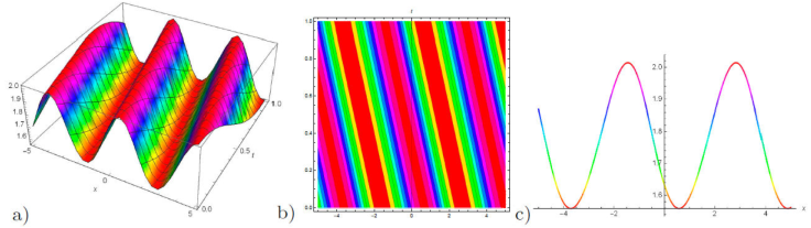
This section contains the graphical depictions of optical solitons and periodic wave structures. A family of periodic and solitary wave solitons are shown for a given set of values. In this section, the graphical representation of exact solution of (3+1)-BLMP model has been illustrated. Soliton solutions, dark solitons, single soliton, periodic type solitons, bell shaped solitons, singular solitons, as well as various Boiti-Leon-Manna-Pempinelli soliton solutions are obtained in various forms. The new (F/G)-expansion method and the unified method is applied to get the exact traveling wave solutions for the set of values. The 3D, contour and 2D graphs visualize the nature of nonlinear waves constructed from Eq. (1).

6. Conclusion

In this study, we have found a large number of exact solutions to the higher-dimensional Boiti-Leon-Manna-Pempinelli model which plays a significant role to describe numerous dynamical phenomenon in diverse disciplines of science and engineering such as chemical physics, particle physics, quantum field theory, optical fibers, fluid dynamics, hydrodynamics. Exact traveling wave solutions always provide a complete account of dynamical behaviour of the most complicated physical phenomena that have yet to be researched. A set of state-of-the-art analytical techniques namely the new (F/G)-expansion method and the unified method are employed to develop numerous solitary and traveling wave solutions such as the bright solitons, dark solitons, single soliton, periodic type solitons, bell shaped solitons, hyperbolic and trigonometric functions, for details see Figs. 1-12. We are able to achieve distinct graphical interpretations to the nonlinear wave structures for the suitable choice of parameters. The contemplated results confirm that the applied techniques are powerful and efficient for obtaining analytical solutions to a variety of nonlinear problems emerging in the contemporary era of ocean engineering and wave motion. In future, other methodologies and nonlinearity laws may be used to explore such model, thus there is still a lot of fresh work to be done on it.

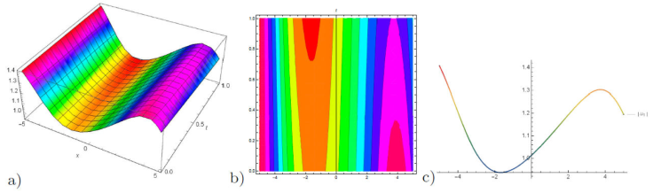
Figure 1 a) 3D plot, b) contour plot and c) 2D plot for the solution of u 1(x, y, z, t) for the values of λ = 0.5, μ = 0.1, and v = -0.4, y = 1. 

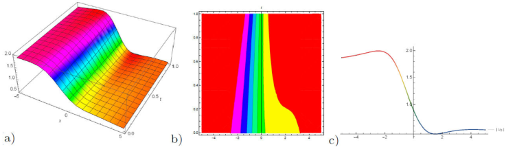
Figure 2 a) 3D plot, b) contour plot and c) 2D plot for the solution of u 3(x, y, z, t) for the values of λ = 0.3, μ = -0.9, and v = 0.7, y = 1. 

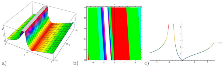
Figure 3 a) 3D plot, b) contour plot and c) 2D plot for the solution of u 7(x, y, z, t) for the values of λ = 0.1, μ = -2.9, and v = 0.5, y = 1. 

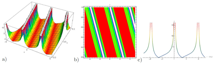
Figure 4 a) 3D plot, b) contour plot and c) 2D plot for the solution of u 8(x, y, z, t) for the values of λ = -1.1, μ = 2.1, and v = 1.4, y = 1. 

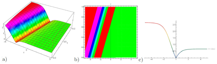
Figure 5 a) 3D plot, b) contour plot and c) 2D plot for the solution of u 9(x, y, z, t) for the values of λ = 1.5, μ = 0.5, and v = -2.7, t = 1, y = 1.  

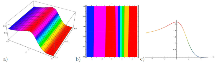
Figure 6 a) 3D plot, b) contour plot and c) 2D plot for the solution of u 11(x, y, z, t) for the values of λ = 1.05, μ = -0.09, and v = -0.05, y = 1, t = 1. 

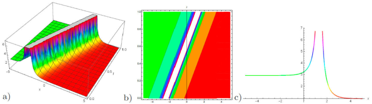
Figure 7 a) 3D plot, b) contour plot and c) 2D plot for the solution of u 13(x, y, z, t) for the values of λ = 1, μ = 0.4, γ = -2.2, κ = -2, and v = 1.2, A = 2, A 0 = 1, η 0 = 1, z = -2, B = -1, y = 1, t = 1. 

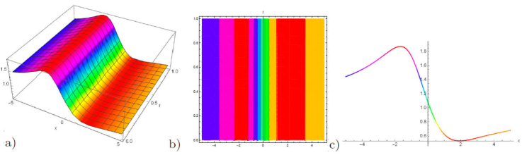
Figure 8 a) 3D plot, b) contour plot and c) 2D plot for the solution of u 15(x, y, z, t) for the values of λ = -0.2, μ = 1.2, γ = 0.02, κ = 2, and v = -0.003, A = -1.02, B = -0.5, A 0 = 1, η 0 = 1, z = 0.1 = y = 1, t = 1. 

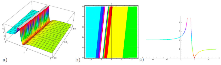
Figure 9 a) 3D plot, b) contour plot and c) 2D plot for the solution of u 19(x, y, z, t) for the values of λ = -0.2, μ = 1, η 0 = 1, z = 1, γ = -0.3, κ = -1, and v = -1, A = -1, A 0 = 1, B = -0.3, y = 1, t = 1. 

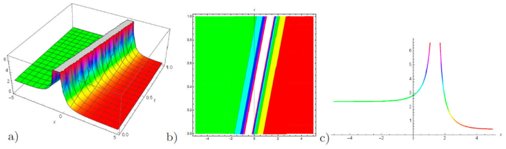
Figure 10 a) 3D plot, b) contour plot and c) 2D plot for the solution of u 23(x, y, z, t) for the values of λ = -0.2, μ = 1, η 0 = 1, z = 1, γ = -0.3, κ = -1, and v = -1, A = -1, A 0 = 1, B = -0.3, y = 1, t = 3. 

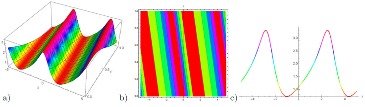
Figure 11 a) 3D plot, b) contour plot and c) 2D plot for the solution of u 25(x, y, z, t) for the values of λ = 0.2, μ = -1, η 0 = 1, z = -2, γ = 4, κ = -1.2, and v = 0.2, A = -1.2, A 0 = 1, B = 1.3, y = 1, t = 2. 

Figure 12 a) 3D plot, b) contour plot and c) 2D plot for the solution of u 30(x, y, z, t) for the values of λ = 0.2, μ = -1, η 0 = 1, z = 4, γ = 1.7, κ = -1.2, and v = -1.2, A = -0.2, A 0 = 1, B = 1.3, y = -3, t = 1. 

References

1. J. C. Heinrich, D. W. Pepper, Intermediate finite element method: fluid flow and heat transfer applications, Routledge (2017). [ Links ]

2. K. O. Lye, S. Mishra, D. Ray, Deep learning observables in computational fluid dynamics, Journal of Computational Physics 410 (2020) 109339. https://doi.org/10.1016/j.jcp.2020.109339. [ Links ]

3. J. Feng, T. Mikami, J. Zimmer, A hamilton-jacobi pde associated with hydrodynamic fluctuations from a nonlinear diffusion equation, Communications in Mathematical Physics 385 (2021) 1-54. https://doi.org/10.1007/s00220-021-04110-1. [ Links ]

4. M. Alquran, M. Ali, O. Alshboul, Explicit solutions to the timefractional generalized dissipative Kawahara equation, Journal of Ocean Engineering and Science (2022). https://doi.org/10.1016/j.joes.2022.02.013. [ Links ]

5. I. Jaradat, M. Alquran, A variety of physical structures to the generalized equal-width equation derived from wazwaz-benjamin-bona-mahony model, Journal of Ocean Engineering and Science (2022). https://doi.org/10.1016/j. joes.2021.08.005. [ Links ]

6. M. Alquran, M. Ali, H. Jadallah, New topological and nontopological unidirectional-wave solutions for the modified-mixed kdv equation and bidirectional-waves solutions for the benjamin ono equation using recent techniques, Journal of Ocean Engineering and Science (2022). https://doi.org/10.1016/j.joes.2021.07.008. [ Links ]

7. M. Alquran, Optical bidirectional wave-solutions to new two mode extension of the coupled kdv schrodinger equations, Optical and Quantum Electronics 53 (2021) 19. https://doi.org/10.1007/s11082-021-03245-8. [ Links ]

8. A. Rani, A. Zulfiqar, J. Ahmad, Q. M. U. Hassan, New soliton wave structures of fractional gilson-pickering equation using tanh-coth method and their applications, Results in Physics 29 (2021) 104724. https://doi.org/10.1016/j.rinp.2021.104724. [ Links ]

9. M. Alquran, Physical properties for bidirectional wave solutions to a generalized fifth-order equation with third-order time-dispersion term, Results in Physics 28 (2021) 104577. https://doi.org/10.1016/j.rinp.2021.104577. [ Links ]

10. X.-F. Yang, Z.-C. Deng, Y. Wei, A riccati-bernoulli sub-ode method for nonlinear partial differential equations and its application, Advances in Difference Equations 1 (2015) 117. https://doi.org/10.1186/s13662-015-0452-4. [ Links ]

11. M. Mirzazadeh, R. T Alqahtani, A. Biswas, Optical soliton perturbation with quadratic-cubic nonlinearity by riccati-bernoulli sub-ode method and kudryashov’s scheme, Optik 145 (2017) 74-78.https://doi.org/10.1016/j.ijleo.2017.07.011. [ Links ]

12. A.-M. Wazwaz, L. Kaur, Complex simplified hirotas forms and lie symmetry analysis for multiple real and complex soliton solutions of the modified kdv-sine-gordon equation, Nonlinear Dynamics 95 (2019) 2209, https://doi.org/10.1007/s11071-018-4686-z. [ Links ]

13. Y. Yildirim, Optical solitons with biswas-arshed equation by sine-gordon equation method, Optik 223 (2020) 165622. https://doi.org/10.1016/j.ijleo.2020.165622. [ Links ]

14. M. A Akbar, et al., Soliton solutions to the Boussinesq equation through sine-gordon method and kudryashov method, Results in Physics 25 (2021) 104228. https://doi.org/10.1016/j.rinp.2021.104228. [ Links ]

15. S. Javeed, S. Riaz, K. Saleem Alimgeer, M. Atif, A. Hanif, D. Baleanu, First integral technique for finding exact solutions of higher dimensional mathematical physics models, Symmetry 11 (2019) 783. https://doi.org/10.3390/sym11060783. [ Links ]

16. H. Yépez-Martinez, J. Gomez-Aguilar, A. Atangana, First integral method for non-linear differential equations with conformable derivative, Mathematical Modelling of Natural Phenomena 13 (2018) 14. https://doi.org/10.1051/mmnp/2018012. [ Links ]

17. M. Mirzazadeh, A. Biswas, Optical solitons with spatiotemporal dispersion by first integral approach and functional variable method, Optik 125 (2014) 5467-5475. https://doi.org/10.1016/j.ijleo.2014.02.042. [ Links ]

18. K. U Tariq, M. Inc, A. Pashrashid, M. Zubair, L. Akinyemi, On the structure of unsteady korteweg-de vries model arising in shallow water, Journal of Ocean Engineering and Science (2022). https://doi.org/10.1016/j.joes.2022.01.011. [ Links ]

19. S. Bilige, T. Chaolu, X. Wang, Application of the extended simplest equation method to the coupled schrodinger-boussinesq equation, Applied Mathematics and Computation 224 (2013) 517, https://doi.org/10.1016/j.amc.2013.08.083. [ Links ]

20. E. M. Zayed, R. M. Shohib, Optical solitons and other solutions to biswas-arshed equation using the extended simplest equation method, Optik 185 (2019) 626, https://doi.org/10.1016/j.ijleo.2019.03.112. [ Links ]

21. E. M. Zayed, R. M. Shohib, A.-G. Al-Nowehy, Solitons and other solutions for higher-order nls equation and quantum zk equation using the extended simplest equation method, Computers and Mathematics with Applications 76 (2018) 2286, https://doi.org/10.1016/j.camwa.2018.08.027. [ Links ]

22. N. M. Rasheed, M. O. Al-Amr, E. A. Az-Zobi, M. A. Tashtoush, L. Akinyemi, Stable optical solitons for the higher-order non-kerr nlse via the modified simple equation method, Mathematics 9 (2021) 1986. https://doi.org/10.3390/math9161986. [ Links ]

23. M. Younis, A. Zafar, The modified simple equation method for solving nonlinear phi-four equation, International Journal of Innovation and Applied Studies 2 (2013) 661, http://www.issr-journals.org/ijias/. [ Links ]

24. Y. Liang, Exact solutions of the (3+ 1)-dimensional modified kdv-zakharovkuznetsev equation and fisher equations using the modified simple equation method, Journal of Interdisciplinary Mathematics 17 (2014) 565, https://doi.org/10.1080/09720502.2014.950054. [ Links ]

25. M. Alquran, R. Alhami, Convex-periodic, kink-periodic, peakon-soliton and kink bidirectional wave-solutions to new established two-mode generalization of cahn-allen equation, Results in Physics 34 (2022) 105257, https://doi.org/10.1016/j.rinp.2022.105257. [ Links ]

26. S. Sahoo, G. Garai, S. S. Ray, Lie symmetry analysis for similarity reduction and exact solutions of modified kdv-zakharov-kuznetsov equation, Nonlinear Dynamics 87 (2017) 1995, https://doi.org/10.1007/s11071-016-3169-3. [ Links ]

27. T.-T. Zhang, On lie symmetry analysis, conservation laws and solitary waves to a longitudinal wave motion equation, Applied Mathematics Letters 98 (2019) 199, https://doi.org/10.1016/j.aml.2019.06.016. [ Links ]

28. E. H. Zahran, M. M. Khater, Modified extended tanh-function method and its applications to the bogoyavlenskii equation, Applied Mathematical Modelling 40 (2016) 1769, https://doi.org/10.1016/j.apm.2015.08.018. [ Links ]

29. Y. Pandir, A. Yildirim, Analytical approach for the fractional differential equations by using the extended tanh method, Waves in Random and Complex Media 28 (2018) 399, https://doi.org/10.1080/17455030.2017.1356490. [ Links ]

30. K. U. Tariq, M. Khater, M. Inc, On some novel bright, dark and optical solitons to the cubic-quintic nonlinear nonparaxial pulse propagation model, Optical and Quantum Electronics 53 (2021) 1-13. https://doi.org/10.1007/s11082-021-03370-4. [ Links ]

31. C. Song, Y. Liu, Extended homogeneous balance conditions in the subequation method, Journal of Applied Analysis (2021). https://doi.org/10.1515/jaa-2021-2068. [ Links ]

32. A. Yokus, H. Durur, H. Ahmad, Hyperbolic type solutions for the couple Boiti-Leon-Pempinelli system, Facta Universitatis, Series: Mathematics and Informatics 35 (2020) 523, https://doi.org/10.22190/FUMI2002523Y. [ Links ]

33. M. Osman, A.-M. Wazwaz, A general bilinear form to generate different wave structures of solitons for a (3+ 1)-dimensional Boiti-Leon-Manna-Pempinelli equation, Mathematical Methods in the Applied Sciences 42 (2019) 6277, https://doi.org/10.1002/mma.5721. [ Links ]

34. M. R. Ali, W.-X. Ma, New exact solutions of nonlinear (3+1)-dimensional boiti-leon-manna-pempinelli equation, Advances in Mathematical Physics 2019 (2019) 9801638. https://doi.org/10.1155/2019/9801638. [ Links ]

35. M. Darvishi, M. Najafi, L. Kavitha, M. Venkatesh, Stair and step soliton solutions of the integrable (2+1) and (3+1)-dimensional Boiti-Leon-Manna-Pempinelli equations, Communications in Theoretical Physics 58 (2012) 785. https://doi.org/10.1088/0253-6102/58/6/01. [ Links ]

36. G.-q. Xu, Painleve analysis, lump-kink solutions and localized excitation solutions for the (3+1)-dimensional boiti-leon-manna-pempinelli equation, Applied Mathematics Letters 97 (2019) 81, https://doi.org/10.1016/j.aml.2019.05.025. [ Links ]

37. X.-L. Gai, Y.-T. Gao, X. Yu, L. Wang, Painleve property, autobacklund transformation and analytic solutions of a variable-coefficient modified korteweg-de vries model in a hot magnetized dusty plasma with charge fuctuations, Applied Mathematics and Computation 218 (2011) 271, https://doi.org/10.1016/j.amc.2011.05.049. [ Links ]

38. Y. Yildirim, E. Yasar, A. R. Adem, A multiple exp-function method for the three model equations of shallow water waves, Nonlinear Dynamics 89 (2017) 2291, https://doi.org/10.1007/s11071-017-3588-9. [ Links ]

39. M. Darvishi, M. Najafi, Application of multiple exp-function method to obtain multi-soliton solutions of (2+1)-and (3+1)-dimensional breaking soliton equations, Am. J. Comput. Appl. Math 1 (2011) 41, https://doi.org/10.5923/j.ajcam.20110102.08. [ Links ]

40. D. Wiedemann, The two-scale transformation method, Asymptotic Analysis (2011) 1. https://doi.org/10.3233/ASY-221766. [ Links ]

41. F. Ebrahimi, M. Ghadiri, E. Salari, S. A. H. Hoseini, G. R. Shaghaghi, Application of the differential transformation method for nonlocal vibration analysis of functionally graded nanobeams, Journal of Mechanical Science and Technology 29 (2015) 1207, https://doi.org/10.1007/s12206-015-0234-7. [ Links ]

42. R. Hanel, S. Thurner, M. Gell-Mann, Generalized entropies and the transformation group of superstatistics, Proceedings of the National Academy of Sciences 108 (2011) 6390, https://doi.org/10.1073/pnas.1103539108. [ Links ]

43. K. U. Rehman, A. A. Malik, M. Malik, M. Tahir, I. Zehra, On new scaling group of transformation for prandtl-eyring uid model with both heat and mass transfer, Results in physics 8 (2018) 552, https://doi.org/10.1016/j.rinp.2017.12.071. [ Links ]

44. M. Mortazavi, M. Gachpazan, New (f/g)-expansion method and its applications to nonlinear pdes in mathematical physics, Electronic Journal of Mathematical Analysis and Applications 4 (2016) 175. http://fcag-egypt.com/Journals/EJMAA/. [ Links ]

45. M. Osman, A. Korkmaz, H. Rezazadeh, M. Mirzazadeh, M. Eslami, Q. Zhou, The unified method for conformable time fractional Schrödinger equation with perturbation terms, Chinese Journal of Physics 56 (2018) 2500, https://doi.org/10.1016/j.cjph.2018.06.009. [ Links ]

46. X. Shi, D. Shi, W. L. Li, Q. Wang, A unified method for free vibration analysis of circular, annular and sector plates with arbitrary boundary conditions, Journal of Vibration and Control 22 (2016) 442, https://doi.org/10.1177/1077546314533580. [ Links ]

Received: February 22, 2022; Accepted: March 17, 2022

E-mail: minc@firat.edu.tr

Creative Commons License This is an open-access article distributed under the terms of the Creative Commons Attribution License