1. Introduction

The study of waves is of great importance in explaining many complex phenomena as tsunami, earthquake, and preventing damages caused by these natural events. Researching and evaluating the effects of global warming can be given as an example for this case. Short-range seismic earthquakes from Mw 6.9 on 8.8 magnitudes in Japan in 2011 are caused by acoustic wave movements and tsunamis in the ocean along the coastal zone [¹]. When the data of this situation are examined, many multidisciplinary fields of study related to the subject have been developed and researches are carried out on how these destructive powers can be transformed into alternative energy sources at present. The marine environment has many wave classifications. SWWs have a wide range of research within these classes. Shallow water is the region that occurs when the length of the wave entering the local water depth is higher than the depth in the region. The orbital motion of the water entering this region is disrupted and they cannot return to the same position again. When waves enter shallow water areas, they begin to be impressed by the ocean bottom, and over time ocean erosion is growing as the shallowness of the environment increases. SWWs refer to flow at the free surface of a body of water in these regions under the influence of gravity or flow under a horizontal pressure surface in a fluid. SWW equations have a form of partial differential equations that are used to express complex events. SWW equations identify the motion of the wavelengths that are short relative to the size of the waves propagating over the water bodies. Also, these equations are used to illustrate the flow of vertically well-mixed water bodies with a horizontal length scale much bigger than the fluid depth [²-⁵]. Many models of physical phenomena in the world are based on nonlinear partial differential equations. Over time, a new perspective on derivatives in this class of equations has been introduced to arrive at more realistic phenomena. Thus, differential equations are started to be expressed with fractional derivatives instead of integer derivatives. FDEs are widely used in applied mathematics, ocean and coastal engineering, mathematical physics, fluid dynamics, metrology, plasma physics, acoustic gravity waves, and other complex areas [⁶-⁸]. It is very important to acquire the solutions of these equations used in these fields created by real-world problems. Among the powerful and effective methods used to achieve analytical solutions, the modified simple equation method [⁹], the generalized Kudryashov method [¹⁰], the improved F-expansion method [¹¹], the new extended direct algebraic method [¹²], the (G’/G)-expansion method [¹³], the ERF method [¹⁴], the first integral method [¹⁵], the modified trial equation method [¹⁶], the generalized exponential rational function method [¹⁷], the generalized bifurcation method [¹⁸], the modified extended tanh-function method [¹⁹], the sub-equation method [²⁰], and so on. However, these methods need some specific definitions to be applied to equations containing fractional order derivatives. Many definitions of fractional derivatives are used in the literature. Riemann-Liouville, Grünwald-Letnikov, Caputo, Jumarie’s modified Riemann-Liouville definitions are widely used fractional derivative definitions [⁷, ²¹-²⁴]. The linearity property is the common feature of all fractional derivative definitions in the literature. In addition, definitions have pros and cons compared to each other. The well-known Riemann-Liouville and Caputo derivative definitions are identified with fractional integrals. Thus, these definitions have some nonlocal features including historical memory and forthcoming dependence [²⁵]. However, these definitions have some disadvantages such as that they do not provide the derivative of the quotient of two functions, the derivative of the product of two functions, the Leibniz rule, Rolle’s theorem, the chain rule, and mean value theorem of a classical derivative [²⁶]. These mismatches have caused many problems in real implementations. Thus, Khalil et al. introduced a new definition of fractional derivatives to overcome these difficulties, and this new definition is named conformable fractional derivative (CFD) [²⁷]. Moreover, Abdeljawad made some very important contributions to the definition of conformable fractional derivative such as right and left conformable fractional derivatives, chain rule for fractional order, Laplace transform, Grönwall’s inequality, exponential function, Taylor power series expansion, and so on [²⁸]. Besides, geometrical and physical meanings of the CFD have been explicated in [²⁹, ³⁰]. This interesting local definition is an extension of the known limit definition of the derivative of a function. Although the local fractional derivatives do not have the memory condition of the nonlocal fractional derivatives, they have gained significant interest recently because they preserve some of the efficient properties of the classical derivative [³¹]. To summarize the main advantages of the proposed definition, the CFD is natural and, unlike other definitions, provides semigroup properties and some important theorems [³², ³³]. It is more understandable and applicable than nonlocal definitions in modeling many complex problems. It is a very useful tool for extending transformations like Laplace, Sumudu and solving some singular differential equations [²⁵]. Since it has a simple and applicable form, it provides great convenience in reaching numerical and analytical solutions of equations. Also, new mathematical tools are needed since real-world problems are getting more complex day by day. This useful definition is used to create and extend new definitions of local derivatives. For instance, Atangana et al. presented a modified version of the conformable derivative which is called beta-derivative [³⁴]. The main objective of this article is to introduce the implementation of the ERF method for obtaining new analytical wave solutions. We study the exact solutions of the nonlinear coupled time-fractional B-B equation [³⁵], the nonlinear time-fractional ALW equation [³⁶], and the nonlinear (2 + 1)-dimensional space-time fractional GNNV equation [³⁷], which are frequently used in fluid dynamics and the propagation of SWWs [³⁸, ³⁹]. There are many inspiring studies in the literature in which these proposed models are constructed with different definitions of fractional derivatives. The analytical solutions of B-B equation have been obtained with the residual power series [⁴⁰] and the first integral methods [⁴¹]. Al-Shawba et al. [⁴²] have also attained several wave solutions of the B-B equation. Then, Fan et al. [⁴³] have used the (G’/G)-expansion method to get the traveling wave solutions. In [⁴⁴-⁴⁷] various effective analytical methods have been performed to the ALW equation and in these studies, various wave solutions have been achieved. Besides, wave solutions of the fractional GNNV equation has been investigated with various analytical methods such as the extended Jacobi’s elliptic function expansion method [³⁷], the improved fractional (D ^α G/G) method [⁴⁸], the (G’/G)-expansion method [⁴⁹], and the generalized fractional subequation method [⁵⁰]. As far as we know, the exact wave solutions we obtained are different from previous solutions of these models. The application of the method is based on that definition of the conformable derivative, traveling wave transformation, and the general form of exact solutions which are expressed in series sum with unknown coefficients and exponential function. The correctness, validity, and graphics of the solutions are obtained. The behaviour of the waves and types of solutions show that the ERF method is a suitable, effective, and innovative technique for finding analytical solutions of fractional equations. The outline of this paper is arranged as follows: In Sec. 2, we give the definition and some basic features of the CFD. In Sec. 3, we describe the major steps of the ERF method. In Sec. 4, the ERF method is implemented in the systems. In Sec. 5, we draw graphs of solutions and give some physical explanations. In Sec. 6, we give some conclusions.

2. Outline of the CFD

The main definition and some characteristics of the CFD are presented in [²⁷, ²⁸].

Definition 1. Given a function q: (0, ∞) → ℝ, the CFD of q order 0 < α ≤ 1 is given as:

If q is α-conformable differentiable in some interval (0, n), n > 0 and

exists then define

Theorem 1. Suppose α ∈ (0, 1], q = q(t) and h = h(t) are α-differentiable functions for all t > 0. Then,

If q is differentiable; then

The chain rule for the CFD proposed in Ref. [²⁸] as follows:

Theorem 2. Let q = q(t) be a α-conformable differentiable and assume h = h(t) is a differentiable function defined in the range of q. Then, the chain rule is given by

Here, we give a short proof of Theorem 2.

Proof. To prove Theorem 2, first we show Eq. (6).

Let μ = t ^α-1 k in Definition 1. Then,

Thus, we have obtained the relation between conformable and ordinary derivatives. Then, using Eq. (6) and the chain rule for the ordinary derivative we can easily observe

This completes the proof.

3. The exponential rational function method

This efficient method was first introduced by [⁵¹] and it has been used to attain solutions of many integer or fractional or der nonlinear models in the literature [¹⁴, ⁵², ⁵³]. Moreover, we express the major steps of the ERF method [¹⁴, ⁵³].

Suppose that nonlinear conformable partial differential equation as follows

where R is a polynomial of u(x, y, t) and its derivatives.

Step 1. We implement the conformable type wave transformation,

and here using the chain rule of the CFD, we convert Eq. (10) into the following ordinary differential equation (ODE):

where the superscripts denote the derivation according to ε.

Step 2. Assume that the general solution form of Eq. (12) can be written in terms of finite series in the following form:

where α _j (α _N ≠ 0) are constants.

Step 3. We evaluate the value of N in Eq. (13) by using the homogeneous balancing principle in Eq. (12).

Step 4. We replace Eq. (13) and all its necessary derivatives into Eq. (12). Then, we get a polynomial of e ^iε and collecting all possible powers of e ^iε (i = 0, 1, 2, …) and equalize all the coefficients of this polynomial to zero. This process ensures to the achievement of the solution cases. As a result of all the major steps of the method, we get exact solutions of the proposed nonlinear equation.

4. Applications

In this section, the ERF method is performed to the system of nonlinear fractional SWW equations.

5. Graphical illustration and explanation

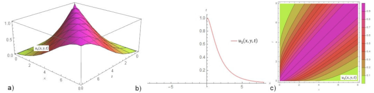
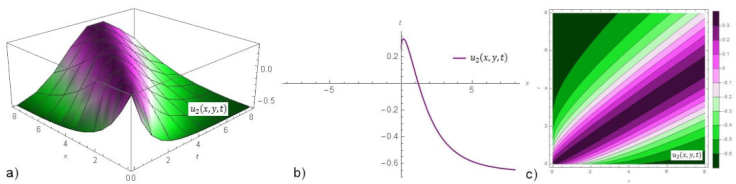
One of the most observable phenomenon in nature is water waves. The study of water waves and their various applications is central to applied fields such as fluid dynamics and ocean engineering. Also, in these areas the behaviours of waves such as breaking of water waves on beaches, ocean waves caused by storms, flood waves in rivers, ship waves on water, movements of free oscillations of water in closed areas like harbours and lakes are studied [⁵⁶]. Examining the non-linear models of these waves in various conditions and presenting their graphs are very important to explain their physical behaviours. Generally, researches of such types of exact wave solutions provide a reason and additional clarification for wave strategies. The solitary waves are specific forms of traveling waves and they protect their permanent structure, even after impact with other solitary waves. Furthermore, the dynamical behaviour of solitary wave types propose the existence of an inclusive theory. Thus, in this section, we determine wave forms and illustrate graphs of the attained exact wave solutions of the proposed equations. We achieve different solution forms such as singular, combo-singular, dark (topological), and bright (non-topological) soliton. The dark solitary waves are more stable and more resistant to impact than other wave forms. It is well known that dark solutions describe solitary waves with density lower than the background, bright solutions whose maximum density is greater than the background, and singular solutions, which are solitary waves with discontinuous derivatives [⁵⁷]. Moreover, Eq. (22)u ₁(x, t), Eq. (24)u ₂(x, t), Eq. (26)u ₃(x, t), Eq. (28)u ₄(x, t), Eq. (37)u ₁(x, t), and Eq. (39)u ₂(x, t) are dark solutions. Eq. (23)v ₁(x, t), Eq. (25)v ₂(x, t), Eq. (38)v ₁(x, t), and Eq. (51)u ₁(x, y; t) solutions have bright wave forms. Eq. (27)v ₃(x, t), Eq. (29)v ₄(x, t), Eq. (40)v ₂(x, t), Eq. (52)v ₁(x, y, t), and Eq. (53)w ₁(x, y, t) are singular soliton solutions. Eq. (54)u ₂(x, y, t), Eq. (55)v ₂(x, y, t), and Eq. (56)w ₂(x, y, t) are combo-singular solutions. The behaviors of these waves can be clearly observed in graphs so that they have various shapes in regard to α and other proper coefficients. The graphs of the solitary waves solutions are sketched in three types as 3D, 2D, and contour graphs. Graphs are plotted on several intervals -8 ≤ x, t ≤ 8, -8 ≤ x ≤ 8 and 0 ≤ x, t ≤ 8, respectively. Further, all contour graphs are drawn using the same values as 3D-graphs. Positive and negative directional wave solutions are included in the same graphs (Fig. 1 and Fig. 2) so that the opposite waves can be clearly observed.

5.1. Graphs of the B-B equation

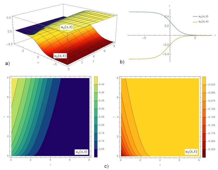
Figure 1 a) 3D-graphs. b) 2D-graphs. c) Contour graphs. Graphs of Eq. (22)u1(x, t) and Eq. (24)u ₂(x, t). 

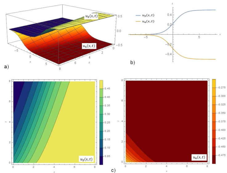
Figure 2 a) 3D-graphs. b) 2D-graphs. c) Contour graphs. Graphs of Eq. (26)u ₃(x, t) and Eq. (28)u4(x, t). 

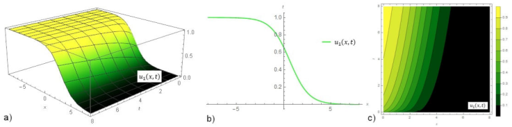
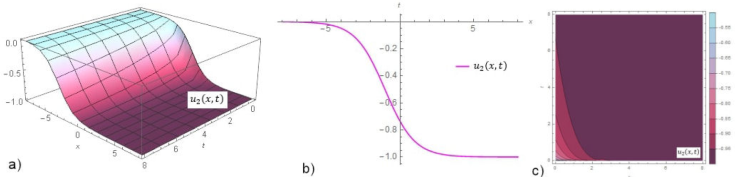
Figure 1a) shows the dark solution for Eq. (22)u ₁(x, t) α = 0.6, ρ = 0.5 and Eq. (24)u ₂(x, t) for α = 0.6, ρ = -0.5. Figure 1b) demonstrates the graph for the above values and t = 0.3. Figure 1c) remarks the contour surfaces of u ₁(x, t) and u ₂(x, t). Figure 2a) indicates the dark solution Eq. (26)u ₃(x, t) for α = 0.8, ρ = 0.5 and Eq. (28)u ₄(x, t) for α = 0.8, ρ = -0.5. Figure 2b) expresses solutions fixed at point t = 0.3 with the cases in a). Figure 2c) specifies the contour surfaces of u ₃(x, t) and u ₄(x, t). Figure 3a) gives the dark solution Eq. (37)u ₁(x, t) for α = 0.4 and ρ = 0.5. Figure 3b) shows this solution for t = 0.2 and the same cases in 3D. Figure 3c) shows the contour graph of u ₁(x, t). Figure 4a)points the dark solution Eq. (39)u ₂(x, t) for α = 0.3 and ρ = -0.5. Figure 4b) is u ₂(x, t) fixed at point t = 0.2 with the same values in a). Figure 4c) indicates the contour graph of u ₂(x, t). Figure 5a) introduces the bright solution Eq. (51)u ₁(x, y, t) for α = 0.6, ρ = -1, k = 1, l = -2, and y = 0. Figure 5b) shows graph of wave solution for the same states in 3D and t = 0.1. Figure 5c) demonstrates the contour graph of u ₁(x, y, t). Figure 6a) manifests the combo-singular solution Eq. (54)u ₂(x, y, t) for α = 0.6, ρ = -1.3, k = 1, 1 = -2, and y = 0. Figure 6b) infers u ₂(x, y, t) for t = 0.1 and the same cases in a). Figure 6c) gives the contour graph of u ₂(x, y, t).

5.2. Graphs of the ALW equation

Figure 3 a) 3D-graph. b) 2D-graph. c) Contour graph. Graphs of Eq. (37)u ₁(x, t). 

Figure 4 a) 3D-graph. b) 2D-graph. c) Contour graph. Graphs of Eq. (39)u ₂(x, t). 

5.3. Graphs of the GNNV equation

Figure 5 a) 3D-graph. b) 2D-graph. c) Contour graph. Graphs of Eq. (51)u ₁(x, y, t). 

Figure 6 a) 3D-graph. b) 2D-graph. c) Contour graph. Graphs of Eq. (54)u ₂(x, y, t). 

6. Conclusion

The ERF method has been performed to the nonlinear time-fractional coupled B-B, ALW, and space-time fractional GNNV equations to obtain new exact wave solutions. Also, fractional derivatives in the equations have been handled in a conformable sense due to their lucidity and applicability. The correctness of these results has been examined by using the Mathematica software. The graphics of the solutions have been constructed under suitable cases and parameters. The obtained results include hyperbolic functions which express various physical states in applied sciences. The hyperbolic-sine emerges in the gravitational potential of a cylinder and in calculating the Roche limit, while the hyperbolic-cosine refers to the shape of a curve formed by a chain, rope, or wire hanging freely from two points not on the same vertical line. Further, the hyperbolic-tangent appears in the calculation of magnetic moment and speed of specific relativity, and the hyperbolic-secant shows up the profile of a laminar jet [⁵⁸]. Besides, the general solution function of the ERF method is expressed by an exponential function which provides a great advantage for finding new exact solutions of equations in complex phenomena. This technique is effective, direct, and innovative for solving systems of differential equations with fractional order. We hope that our results contribute to future studies for the behaviour of SWWs used in the fields such as mathematical physics, applied mathematics, ocean engineering, civil engineering, port, and coastal construction.