1. Introduction

Deploying sensors and sensing technology has many benefits, including predictive and preventive maintenance. Continuous, real-time data from assets and processes gives a more holistic view of the technology enterprise. Key benefits of sensors include increased sensitivity in data collection and continuous real-time analysis. Continuous advancements in sensor technology have led to the emergence of smart and intelligent sensors. Smart sensors are capable of detecting conditions for real-time decision making. This approach will help to achieve the Sustainable Development Goals (SDGs) set out by the United Nations [¹].

It is obvious that due to the rapid growth of the world's population, the demand for food will increase significantly in the coming years [²]. Traditional farming methods can no longer meet the growing demands and most importantly they use resources such as land, water, herbicides and fertilizers rather inefficiently. For the most efficient and sustainable use of resources to increase production, automation in agriculture needs to be introduced. The way people and machines work on farms has changed thanks to the integration of the Internet of Things (IoT) with numerous sensors, controllers, and communication protocols.

These sensors can continuously produce a significant amount of data about the condition of crops or animals on farms. The architecture and established analysis of IoT data in agriculture helps select IoT technologies for specific applications [³]. Improving the processing of raw data is one of the requirements that research must address when designing data collection systems based on IoT devices to improve overall system performance. Additional goals are to increase battery life and minimize information loss during data transmission when using wearable devices [⁴].

Sensors play a crucial role by detecting and measuring the values of various parameters such as temperature, pressure, humidity, flow rate, movement and position, and the concentration of certain components in the mixture. They convert physical signals into electrical signals and provide information to the control system in real time, thus making production intelligent and automated. In addition to those already mentioned, there is another promising use of sensors - their medical applications, for example, for routine exhaled air diagnostics. For example, an "electronic nose" design based on a hybrid sensor has been developed to detect the initial stages of lung cancer by analyzing breathing [⁵].

Lung cancer has the highest mortality rate of all cancers in the world, but its early detection significantly increases survival rates. The authors [⁵] proposed two different types of e-noses based on quartz microbalance (QCM) modified semiconductor coatings. Quartz microbalance (QCM) modified with Ag⁺-ZSM-5 zeolite has been proposed for diabetes diagnosis [⁶]. Such a sensor is used to determine the concentration of acetone in the exhaled air of diabetics, since the breath of diabetics and healthy people is clearly distinguishable. Using exhaled gas to diagnose and monitor human disease has numerous advantages for being non-invasive, convenient and environment friendly [⁷].

For the interaction between the automatic systems and the controlled system to take place, the use of sensors is required. During this process, the information they generate must be able to be interpreted by the computer systems that acquire, store and process the information, preferably in real-time. In this sense, there is a process of quantifying the signal generated by the sensor. It is at this stage that it is of interest to be able to estimate the value of the useful signal with the required accuracy, while respecting time constraints, thereby guaranteeing an adequate control of the system of interest [⁸]. In order to meet the time constraints, the algorithm for approximating the desired signal must meet certain characteristics. That is, that it must be easy to implement, and its execution time must be small compared to the time constraints of the system [⁹].

Sensors are the initial source of information about the environment that the control system has, and these devices can be classified in different ways. In particular, given the output signal they generate, the sensors can have outputs that generate signals with voltage, current or frequency, etc. Thus, a way of quantifying the signals generated by the sensors may be improved to improve the performance of the entire system. In the case of signals in the frequency domain, there is a high stability and accuracy in the conversion of the input signal to the sensor output signal. It is for this reason that frequency domain sensors are of interest in various modern applications.

Various methods are known for approximating the frequency of interest, including methods based on counting pulses or periods, or methods based on spectral analysis of the signal, such as methods using the Fourier transform [¹⁰], [¹¹], [¹²], [¹³].

Although each of these methods has its own advantages and disadvantages, as well as its specific applications, in recent years, another method has been proposed and studied, which allows to reduce the measurement time while improving the accuracy of approximation to the measurand; this is the principle of rational approximations [¹⁴], [¹⁵], [¹⁶], [¹⁷]. In this method, the signal to be measured is compared with a reference signal. Before the comparison, both signals are conditioned, and during the comparison, both signals are multiplied in time. А third coincidence signal is generated, in which there are coincidence pulses that are generated during the time while the pulses in the input signal are true. After the first matching pulse, the pulses in the input signals are counted, and then an approximation to the desired frequency can be calculated by knowing the counted pulses and the value of the reference frequency. It has been shown that it is the value of the latter that affects the time required to obtain the best approximation to the measurand. Even so, the relationship between the value of said variable and the error observed in the approximation to the measurand is not completely clear.

In this paper, the aim is to investigate this dependence, and as a consequence, to elucidate the best method for choosing the value of the reference frequency that allows to minimize the error in the measurement process. For this purpose, we will analyze the data generated experimentally in the process of frequency measurement for the signal generated by a sensor that works under the direct piezoelectric effect; further they will be compared with the theoretical model of the measurement process implemented in the course of computational simulation.

2. Background

In nowadays technology, sensors are a source of information that allows computers to have the necessary data for automated decision making. In this regard, improving the accuracy of the data will provide a better understanding of the process scenario in which the sensor is operating. There are different methods for estimating the desired frequency; in general, it can be said that depending on the type of signal, certain methods are used. For example, different methods are used for electrical and optical signals. In the case of electrical signals, the objective of the measurements is to be as fast and accurate as possible [¹⁸]. The methods reported to solve this task should have a minimum measurement time; at the same time, if a more accurate approximation to the measurand is required, a longer time is needed to obtain a satisfactory signal.

In case of optical sources, frequency approximation systems based on Mach-Zehnder interferometers are used [¹⁹]. In the work of Li et al. [²⁰], variations on relative phase shifts are used through an optical delay line and spacing between antennas. Then the phase comparison based on a multi-base line eliminates the ambiguity of the angle of arrival over a large frequency range. Hence, the frequency and angle of arrival are determined by analyzing the phase shift of the intermediate frequency signal. Considering the technological applications of sensors these days, frequency measurement systems are being integrated into embedded systems. For example, an IoT based system has been proposed for vibration analysis by Kneifel et al. [²¹]. In such a system, frequency measurement is done after realizing fast Fourier Transform.

In case of methods based on pulse counting, the principle of rational approximations has been exhaustively studied in the last years, as a result, plenty of mathematical formalisms has been provided for explaining the functioning of such a method, and experimental prototypes have been built for experimental evaluation.

As has been reported [¹⁴], the principle of rational approximations requires enough time to yield a good approximation, which is based on reaching numerator in the form of “one with r zeros”. Later, theoretical advances included the understanding of the pulse width effect in the reduction of error [¹⁵], [¹⁶]. Then, the phase effect and the relation with the shape of error during measurement was discovered [¹⁷]. In these reports, the authors present evaluation of the measurement process of signals with an unknown frequency, then another problem came up; when the signal from sensors has a frequency value that changes from one value to another, there is a frequency shift, then, there are two unknown frequency values. So, with the aim to solve this problem, a formalism to solve the problem of measuring the frequency shift was proposed [²²], [²³], [²⁴], [²⁵].

It is based on measuring the desired or unknown frequency before and after the stimulation of the sensor, then the difference between both measurements is computed. There are two restrictions before this task can be performed, the first is that the approximation to desired frequency must be achieved in a time as short as possible, this with the aim to quantize the frequency variations caused by input stimulus.

The second restriction is related to the uncertainty that is adequate for the sensor, this is that if the frequency shifts generated by the sensor are below of the uncertainty during the measurement, then, there is no relevant information during the measurement process. This is an important aspect, in particular for piezoelectric sensors with a variation of their proper frequency of several parts per million [²⁶]. From the study of the principle of rational approximations, experimental implementations of this method have been proposed.

In particular, the application of this method for the quantification of frequency shifts generated by a quartz crystal has been explored [²⁷], [²⁸]. And also, different applications have been proposed, i.e. the automotive [²⁹] and aerospace industries [³⁰], [²⁴]. A proper understanding of this method would allow its application for improving other instruments that are of current use, for example, frequency response analyzers, such as the used on materials science for studying the nature of nanoparticles [³¹], [³²], [³³], [³⁴].

As this brief revision has shown, different aspects of the principle of rational approximations have been studied, but there are some questions to address before this method can be fully understood. For this reason, in this work, the data generated during the frequency measurement process is evaluated. The signal coincidence process and the measurement method are simulated. This is done with the aim to evaluate the impact of the best coincidences in the frequency measurement process.

3. Methodology

As discussed in other reports [¹⁶], [²²], [²³], the principle of rational approximations allows to estimate an unknown frequency 𝑓_𝑥 (Hz) from data obtained during a signal comparison process. This is that given a reference signal 𝑆₀(𝑓₀) with a known frequency 𝑓₀ (Hz) and a desired signal 𝑆_𝑥(𝑓_𝑥), a third signal 𝑆_𝑥&𝑆₀ can be generated when both signals are multiplied in time. Then, an approximation 𝑓_𝑥 to the true value 𝑓_𝑡 (Hz). This is true if the pulse width of pulses in both signals is considered to have the same duration 𝜏, and 𝜏 ≤ 𝑇₀/2. This is that both signals must have squared pulses with constant duration.

If these conditions are fulfilled, during the signal coincidence process, the pulses are counted since the first coincidence, then the number of pulses from desired 𝑃_𝑛 and reference 𝑄_𝑛 signals are registered in each 𝑛 − 𝑡ℎ coincidence, this, 𝑃_𝑛 and 𝑄_𝑛 denote the amount of pulses counted until the 𝑛 − 𝑡ℎ coincidence for desired and unknown signals respectively. This process is depicted in Fig. 1.

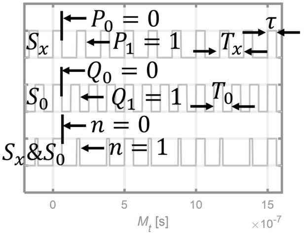
Figure 1 Theoretical measurement process. When 𝑃₀ = 𝑄₀ = 𝑛 = 0, the counting of pulses starts, this is shown in the next coincidence when 𝑛 = 1, where 𝑃1 = 𝑄1 = 1. In addition, it can be noted that 𝑇𝑥 > 𝑇0, which implies that 𝑓𝑥 < 𝑓0. In this method, for both input signals, 𝑆₀ and 𝑆𝑥, 𝜏 has the same duration. 

Then, according to previous reports [¹⁴], [¹⁸], [³⁵], [³⁶], [³⁷], the desired frequency 𝑓_𝑥 can be approximated from the counting of desired and reference signals as.

If the true value 𝑓_𝑡 in Hz of desired signal is known, the relative error 𝛽 is given by

and the measurement time 𝑀_𝑡 (s) by

In this work, a reference signal with a frequency 𝑓₀ was used as reference standard. Different frequency measurement processes were simulated after the use of algorithms proposed in previous reports [²²], [²⁷]. The value of 𝑓_𝑡 was set to 9 MHz, and the measurement process was evaluated with 𝑓₀ = {10, 11, 12, … , 19, 20} MHz. A pulsewidth 𝜏 = 2/(20 × 10⁶) s was used. The algorithms were implemented in MATLAB R2023a.

The results of simulations were evaluated using MATLAB and they are compared with experimental and theoretical results found in related literature. This with the aim to understand the effect of the value of reference frequency in experimental and theoretical results.

4. Results and discussions

The results of direct frequency measurement are presented in Fig. 2. As it can be noted, apparently, all the frequency measurement processes converge to the same frequency value.

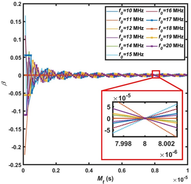
Figure 2 Frequency measurement process under variations of time-reference, variation of relative error 𝛽 during the measurement time 𝑀𝑡, different values of reference frequency 𝑓₀ were considered. The inset shows a zone of interest in 𝑀𝑡 = 8 µs, where there is a transition of positive to negative values of 𝛽. 

This means that the relative error decreases over time. Although there are similar convergence processes, the way each series converge differs. This can be explained as the result of how the coincidences appear. For example, we can consider the first terms of the succession, in case of 𝑓_𝑜 = 10 MHz.

and for 𝑓₀ = 11 MHz,

After the use of Eq. 1, it can be easily shown that the approximated frequency in each case achieves an exact value when 𝑛 = 4, this is that 𝑓_𝑥 = 𝑓_𝑡. In this regard, the coincidences are occurring without interruption, and the value of 𝑛 indicates when the counting of pulses started.

For the process of pulse coincidence, both partial and perfect coincidences generate a packet of coincidences, which groups a finite number of coincidences where a variation in the coincidence time 𝑡_0𝑥 (s) has a particular behavior. These packets appear at a regular rate in 𝑆_𝑥&𝑆₀, and the best approximations yields to a zero error. This is shown in Fig. 2 as the zero crossings of 𝛽.

For almost all the values of 𝑓₀, there is a value in the measurement time, where there is a crossing from positive to negative values of 𝛽 or vice versa. In case of there is no transition to positive values, the value of 𝛽 is cero and it is a constant value during all the 𝑀_𝑡. This means that the crossing point, in case of 8 µs for Fig. 2, occurs at 𝛽 = 0, which is known to occur when a perfect coincidence occurs.

It is noted that the zero crossings, as the shown in the inset of Fig. 2, occur a regular rate, but with a reduction in the magnitude of relative error |𝛽|. As a consequence, at the beginning of measurement process the greatest values of |𝛽|, but different measurement processes yield either positive or negative values of 𝛽, which is known to be caused by the phase of input signals [¹⁸]. For this experiment, the phase condition of both signals was supposed to be the same, this is that both signals, during the measurement process, start at the same time. However, since the first coincidence is not defining the starting value of 𝛽, then it can be attributed to the second coincidence, as shown in Fig 1, where a pulse from a signal starts before the pulse of the other signal where the coincidence exists. This allows us to understand that with enough coincidences, the phase conditions can be obtained even when the signals are supposed to be in the same phase condition. Then, the phase conditions cannot be attributed only to the first coincidence, but to the cumulative effect of all the occurring coincidences during the measurement process.

For these reasons, the phase of input signals defines the number of pulses that exists until the second coincidence (𝑛 = 1). In other words, if there is a perfect coincidence, then 𝛽 = 0, which is true for all cases except at the first packet of coincidences, where 𝑃₀/??₀ = 0/0. Since the packets of coincidences appear at a regular rate, we could think that the rate of variations in the coincidence time 𝑡_0𝑥 is also periodical. This is presented in Fig. 3.

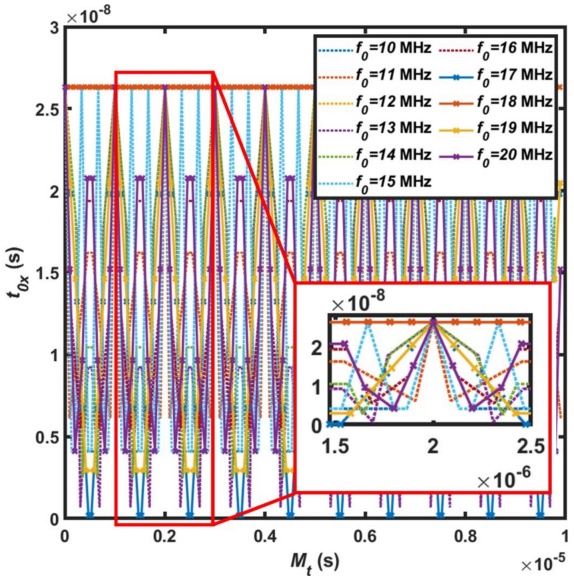
Figure 3 Variations in the coincidence time during frequency measurement process: variations in the time of coincidence 𝑡₀𝑥 are periodical. 

If both signals have the pulse starting and ending at the same time, there is a perfect coincidence, and if one pulse in one signal starts before the pulse from other signal, there is a partial coincidence. This process generates variations on the coincidence time, and the periodicity in this process allows to understand where the best coincidence occurs. As a result, if there are more “perfect” than partial coincidences, then, the average relative error will decrease. It is known that a reduction in the duration of pulse width yields a decrease in the number of partial coincidences. However, during the coincidence process we can identify two types of ratios, the first scenario: 𝑃_𝑛/𝑄_𝑛 = 𝑃_𝑛+??/𝑄_𝑛+𝑚, where 𝑚 > 𝑛; and the second scenario: 𝑃_𝑛/𝑄_𝑛 ≠ 𝑃_𝑛+𝑚/𝑄_𝑛+𝑚, where 𝑚 > 𝑛. In the first scenario, after the 𝑛 − 𝑡ℎ coincidence, there is another coincidence that occurs after 𝑚 subsequent coincidences, where both resulting fractions have the same value. If this is the case, then Eq. 1 would yield the same value.

This is only true when 𝛽 = 0, in Fig. 2 represented by the zero crossings, and in Fig. 3 by the coincidences with the longest duration.

In case of the second scenario, there are partial coincidences that could lie at any moment between two perfect coincidences, but the 𝑃_𝑛+𝑚/𝑄_𝑛+𝑚 value will decrease more as greatest is the difference between 𝑚 and 𝑛, this while the minimum uncertainty is not reached. Unlike relative error, the effect of 𝑚 is not the same in the duration of coincidences, where there are a number of coincidences with the same duration, at least, as the number of packets in the measurement process. These statements imply that the values of 𝛽 that are unlikely to repeat, but the values of 𝑡_0𝑥 certainly are.

Then the relative error is affected by the time where the 𝑃_𝑛/𝑄_𝑛 occur, but not by the coincidence time. This means that when 𝑛 increases, then, the ratio 𝑃_𝑛/𝑄_𝑛 converges to a value, which is approximately 𝑓_𝑥 /𝑓₀, and if the pulse width decreases, then the number of coincidences decreases. In other words, considering two measurement processes with the same 𝑀_𝑡 but different 𝜏. Then the process with the longest 𝜏 will have more coincidences than the other case. This has quite important implications for the experimental implementation of the principle of rational approximations. In this sense, when the number of pulses is too high within a given time, the counters corresponding to 𝑃_𝑛, 𝑄_𝑛 can be overflown, and as a consequence, poor information from the measurement process is obtained, then the steady state could not be achieved. In this case, the number of coincidences is known to occur when the duration of the pulse width increases, or when the values of desired and reference frequency are too close among them.

When studying the coincidences, if the pulse width is too narrow, a number of outcomes could occur. For example, the pulses from 𝑆_𝑥 and 𝑆₀ could not be detected by the circuits used in the physical realization. Since the coincidence time is bounded by 0 < 𝑡_0𝑥 ≤ 𝜏, then the pulses from 𝑆_𝑥 and 𝑆₀ generate a coincidence 𝑆_𝑥&𝑆₀ with a duration lower or equal to 𝜏, and in case of the electronic circuits, they have a minimum time where they are able to detect a logic level as high. As a result, some of these coincidences are not registered because they cannot be detected.

In Fig. 4 the average of the magnitude of relative error |𝜇_𝛽| is presented for each value of reference frequency 𝑓₀.

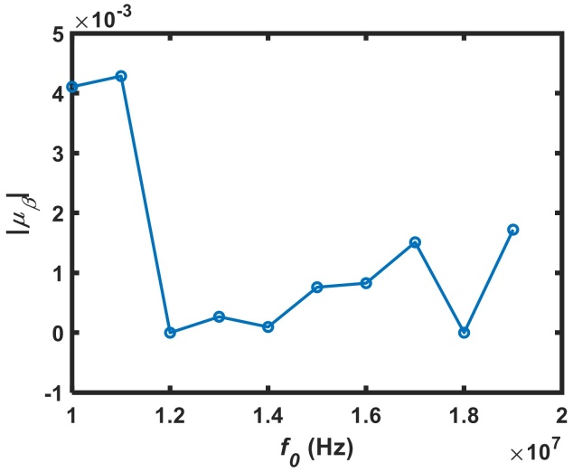
Figure 4 Average magnitude of relative error in frequency measurement process, it is observed that there is a decrement in relative error when the reference frequency increases. 

From Fig. 4, it is observed that when 𝑓₀ = 12 and 18 MHz, |𝜇_𝛽| = 0, which implies that 𝛽 = 0 or 𝑓_𝑥 = 𝑓_𝑡. After Eq. 1, it follows that in each case,

which for 𝑓₀ = 12 MHz, 9/12 = 3/4. And also, in case of 𝑓₀ = 18 MHz, 9/18 = 1/2. No other similar behavior is observed with the other frequency values, which is an indicative that when these rational numbers are formed, there are only the same kind of coincidences, and also, the best approximations to measurand are observed.

4. Conclusions

In this work, the effect of the reference frequency on the estimation process of the signal’s unknown frequency was evaluated. As a result, it was observed that from all the values examined in this study, only in two values the obtained error was zero. This has been found to be cause of the number of pulses in the packets of coincidences, the phase of input signals, and the ration of unknown and reference frequency. However, in general, there was a decrement in the relative error after an increase in the reference frequency. This can be associated with the apparition of more coincidences, which leads to a more populated packets of coincidences. Hence, the present results allow to define the better value of the reference standard that can beused, this when the range of frequencies generated by a sensor is known.