


 nueva página del texto (beta)
 Inglés (pdf)
 Artículo en XML
 Referencias del artículo
 Enviar artículo por email
 Citado por SciELO
  Similares en
SciELO
Similares en
SciELO 
 Permalink
The use of wild plants is often considered necessary, particularly in rural communities that rely heavily on these resources for subsistence. However, the impact of this usage on plant populations is rarely assessed unless there is doubt about the safety of these practices (Hall & Bawa 1993). In Mexico, human communities have a long tradition of utilizing wild plants from arid and semi-arid environments. The genus Agave is the most prominent among these plants, with 159 species accounting for 75 % of its global diversity (García-Mendoza et al. 2007, González-Medrano 2012).
Around 61 % of the species found in Mexico are exclusive to the country. This is because of the diverse nature of the land and the unique characteristics of each species, such as their genetic adaptability, ecological tolerance, and ability to disperse, as well as their interactions with other living beings such as pollinators. Furthermore, geological and climate events that occurred in North America in the past also shaped the current distribution of these species (Pinkava & Baker 1985, Valverde et al. 1996, Good-Avila et al. 2006, Flores-Abreu et al. 2019, Jiménez-Barrón et al. 2020, Eguiarte et al. 2021).
Agaves are highly diverse in Mexico, both in terms of their morphology, phylogeny, and evolution, as well as culturally, as humans have learned to derive benefits from them. Their significance is such that there are approximately 107 species in Mexico that are currently being used in some way (García-Marín et al. 2017).
Agave applanata Hort. ex K.Koch., commonly known as “maguey de ixtle”, “maguey blanco” or “maguey cenizo”, is distributed in semi-arid areas and dry tropical and temperate forests of Guanajuato, Hidalgo, Oaxaca, Puebla, Querétaro, Tlaxcala, and Veracruz (García-Mendoza 2007, Vázquez-García et al. 2007). Despite its being relatively uncommon in its expected range, humans have likely dispersed this species towards the southwest and north of the country, where some isolated populations have been discovered. These populations may have interbred with A. durangensis (Gentry 1982).
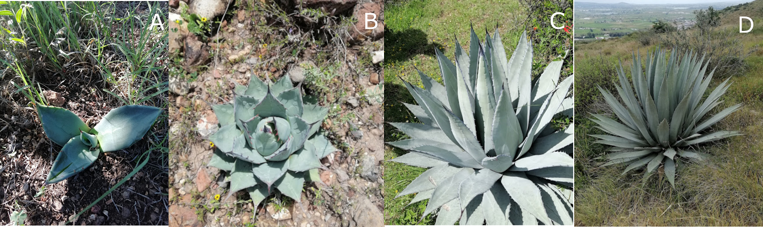
It is a medium-sized agave with broad, flattened, rigid, lanceolate blue-green leaves, the lateral teeth are prominent, dark, and slightly curved at the margins, the terminal spine or mucro is long and rigid, its rosette dies several months after fruiting (Figure 1A), so for a long time the leaves remain turgid (Gentry 1982, Simcha 2017, Casas et al. 2019, García-Mendoza et al. 2019). This agave is in the category of Least Concern (LC) based on IUCN criteria, because its populations and range are relatively large (Casas et al. 2019). According to Mexican legislation NOM-059 (SEMARNAT 2010), it is not in any risk category. In Hidalgo, populations are known in the municipalities of Pachuca, San Agustin Tlaxiaca, Singuilucan, Tezontepec de Aldama, Tulancingo, and Zapotlan (GBIF 2021).
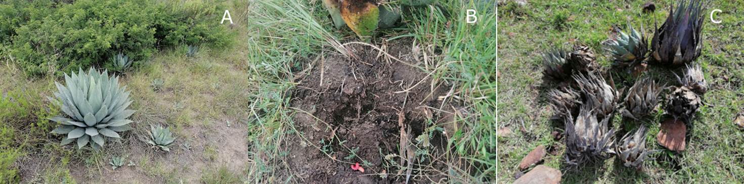
Photographs: MAGM.
Figure 1 Agave applanata. A) Individuals in Hidalgo. B) Chinicuiles and individual turned over for collection. C) Magueyes possibly used in the collection of chinicuiles.
A. applanata is particularly significant for the economy of the state of Hidalgo in Mexico. This is because it provides a habitat for the larva of a type of nocturnal moth called “chinicuil” or “agave red worm” (Comadia redtenbacheri Hamm., Lepidoptera: Cossidae), which has long been used in traditional Mexican cuisine (Montiel 2008, Llanderal-Cázares et al. 2017, Figure 1B). During the rainy season, female moths lay masses of approximately 118 eggs at the base of maguey stalks. The female moth dies after depositing the eggs, and after 30 to 35 days, the eggs hatch. When the larvae emerge, they create galleries inside the stem or rhizome of the agave, where they complete their development (Camacho et al. 2003, Hernández-Livera et al. 2005, Llanderal-Cázares et al. 2017). Usually, people harvest the larvae from maguey plants that are not more than 30 cm high. However, to obtain the largest number of larvae, it is necessary to uproot the entire maguey and remove the stalks and the whole stem, which unfortunately causes the death of the plant (Espinoza-García et al. 2018). Some collectors attempt to replant the maguey, but the success rate is usually low (Esparza-Frausto et al. 2008, Figure 1C).
It is believed that the increasing demand for chinicuiles from both domestic and international markets has had a detrimental effect on the host because the larvae are collected extensively from wild maguey populations. Furthermore, the number of insects that can be gathered has decreased, likely because of overexploitation and predation of larvae, which disrupts their life cycle (Esparza-Frausto et al. 2008). Several solutions have been proposed to address this. These include managing in protected natural areas, choosing a specific stage of development of the plant, and cultivating magueys in greenhouses to facilitate the study of the different larval stages of the insect and its interaction with the agave host (Serrano 2023). The aim of this study was to assess eight populations of Agave applanata, both with and without chinicuil extraction, and to examine other disturbance factors in these locations to determine the impact of human activities on the populations. Harvesting chinicuil is expected to reduce agave's population growth rates. However, the effect on sexual and asexual reproduction is not anticipated to be equal. This is because harvesting occurs on juvenile individuals, who do not reach reproductive size but can still propagate vegetatively.
Material and methods
Study area. One population was analyzed in Oaxaca, one in Guanajuato, one in Querétaro, and five in Hidalgo (Table 1, Figure 2). All are between 2,200 and 2,700 m asl, characterized by arid and semiarid climates and vegetation, including xerophytic scrub, grasslands, and transformed landscapes (companion species belonging to genera Acacia, Agave, Cenchrus, Chloris, Dasylirion, Mammillaria, Melinis, Opuntia, Pinus, Prosopis, Quercus, Schinus and Yucca, to mention a few). In addition, some of these populations are found in the middle strata and/or on the slopes of the surrounding hills.
Table 1 Geographic location of the A. applanata populations analyzed. No: number of population. Pop.: Population name.
| No | Pop | ID | State | Latitude | Longitude |
|---|---|---|---|---|---|
| 1 | Mambru | Mam | Hidalgo | 20.0355833 | -98.93571667 |
| 2 | Zapotlan | Zap | Hidalgo | 19.9699833 | -98.88761667 |
| 3 | San Agustin Tlaxiaca | SAT | Hidalgo | 20.0894667 | -98.86791667 |
| 4 | Pachuca | Pach | Hidalgo | 20.137447 | -98.749657 |
| 5 | Tulancingo | Tul | Hidalgo | 20.11751 | -98.36472 |
| 6 | Tepelmeme | Tep | Oaxaca | 18.0097167 | -97.35935 |
| 7 | Cadereyta | Cad | Querétaro | 20.68113 | -99.800857 |
| 8 | Mineral de Pozos | Min | Guanajuato | 21.1731167 | -100.5036667 |
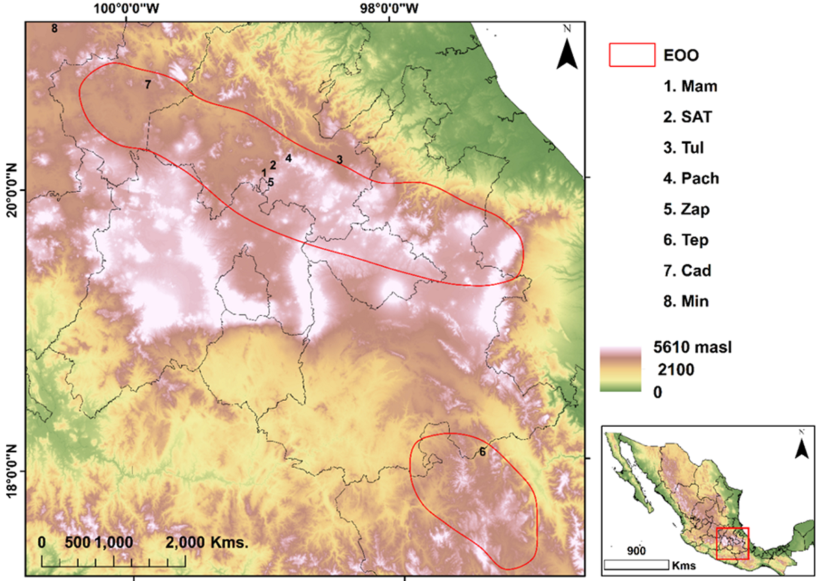
Figure 2 Agave applanata populations considered for this study. The red polygon indicates the estimated extent of occurrence. m asl: meters above sea level. 1) Mambru (Mam). 2) San Agustin Tlaxiaca (SAT). 3 Tulancingo (Tul). 4) Pachuca (Pach). 5) Zapotlan (Zap). 6) Tepelmeme (Tep). 7) Cadereyta (Cad). 8) Mineral de Pozos (Min).
Evaluation of the disturbance. Twelve disturbance indicators according to Martorell & Peters (2009) were evaluated in 50 × 1 m, three transects per site, corresponding to three categories: human activities (evidence of extraction, use, and deterioration of human manipulation.), livestock activity (evidence of grazing, compaction, or browsing by farm animals), and habitat deterioration (evidence of grazing, compaction, or browsing by farm animals). By adding the attribute “Rosette Corpses” to the indicators, dead, turned, dried and discarded individuals with signs of removal were identified, these were likely caused by the collection of chinicuiles (Table 2). The extraction percentage (Ext) was calculated as:
Table 2 Attributes considered for disturbance analysis in eight populations of A. applanata considered in this study. Taken and modified from Martorell & Peters, 2009.
| Category | Disturbance parameter | Symbol |
|---|---|---|
| Human activities | Cutting | w |
| Human activities | Evidence of fire | f |
| Human activities | Roads used by humans | tb |
| Human activities | Distance to the nearest town in m | p |
| Human activities | Distance to human activity centers in m | a |
| Human activities | Corpses | Cad |
| Livestock activity | Herbivory | b |
| Livestock activity | Cattle manure | dc |
| Livestock activity | Roads used by livestock | tt |
| Habitat deterioration | Erosion | e |
| Habitat deterioration | Islands without vegetation | i |
| Habitat deterioration | Completely modified surface | m |
The number obtained estimates the percentage of the population that is used to obtain chinicuiles. A total of 15 polygons were evaluated: two in Mambru (Mam), two in San Agustin Tlaxiaca (SAT), two in Tulancingo (Tul), one in Pachuca (Pach), three in Zapotlan (Zap), all in Hidalgo, two in Tepelmeme, Oax (Tep), one in Cadereyta, Qro (Cad), and two in Mineral de Pozos, Gto (Min). The average area of these polygons was 34,509.5 ± 12,000 m2 , they varied depending on population density and aggregation. The area affected by each disturbance indicator was calculated. A Linear Discriminant Analysis (LDA) was carried out in the R program with the MASS package (Venables & Ripley 2002) to determine the variables affecting the populations in greater proportion, and the impact was presented as a percentage of comparative disturbance (di). This classification method uses qualitative variables to assign cases to two or more groups. It estimates the probability that an observation, given a value of the predictors, belongs to each of the classes of the qualitative variable using Bayes' theorem. The observation is assigned to the class for which the predicted probability is highest (Xanthopoulos et al. 2013).
Classification. To create the static life tables, the heights and two diameters measured at ground level, of 397 A. applanata rosettes from eight different populations were measured. All observed sizes in the field were considered, measured with a tape measure from the ground to the highest point of the plant (cm). Using this data, a clustering analysis based on Euclidean distances using Ward’s method was carried out to obtain a dendrogram and determine the optimal number of categories that best represent the data structure. Ward's minimum variance method calculates the distance between cluster members and the centroid. The centroid of a cluster is defined as the point at which the sum of squared Euclidean distances between the point itself and each other point in the cluster is minimized (Ward 1961).
Subsequently, a k-means clustering was carried out to describe length indicators by group and identify individuals in each population category (Lloyd 1982) The K-means algorithm is a simple iterative clustering algorithm. It uses distance as the metric and calculates the mean distance given the K classes in the dataset. It then assigns each data point to the nearest centroid, creating new centroids for each class. The algorithm uses Euclidean distance as the similarity index for dataset X containing n multidimensional data points and aims to divide the data into K clusters. The goal of clustering is to minimize the sum of the squared distances; in other words, it seeks to reduce the sum of squared distances (Yuan & Yang 2019). Both analyses used the Factoextra package (Kassambara & Mundt 2020). To visually represent the distribution of length categories in each population, a correspondence analysis (CA) was carried out using the FactoMineR package (Lê et al. 2008). All this was done using the R programming language (R Core Team 2022).
Static life tables and survival curves. The average number of seeds per sexually reproductive adult in each population belonging to the Adult 2 category was obtained from field counts to determine fecundity per category (mx). The number of viable (black) and non-viable (white) seeds per fruit, the number of fruits per panicle, the number of umbels per panicle, and the number of panicles per peduncle were counted (Font Quer 1993). Using these values, total seed production per population was estimated and multiplied by the number of sexually reproductive individuals (Adult 2) (Carabias et al. 2009). Other parameters as lx (survival probability), dx (mortality), mxlx (survival of reproductive individuals) Xlxmx (reproductive contribution by class), ex (life expectancy), λ (population growth rate), and R0 (net reproductive rate) were calculated according to Jones (2021). Additionally, individuals with vegetative reproduction (Adult 1) were counted in each population. In this case, mx represents the quantity of clonal offspring. Both Adult 1 and 2 individuals were part of this category, since both can generate this type of propagation. We contrasted the demographic aspects calculated from the vegetative and sexual data using Chi-square tests, excluding null values in SAT, and transforming λ in percentage.
Finally, to create survival curves for each population, data from the lx of the life table that was constructed using sexual reproduction was utilized, we did not use the vegetative matrix because no individuals smaller than 20 cm were found, creating a gap in the transitions between the two initial categories. The data was then transformed to a logarithmic scale and plotted on the Y-axis, while the size category was plotted on the X-axis, like another long-live plants (Gurevitch et al. 2006). This plot was drawn using the ggplot2 package (Wickham 2016), part of the R programming language (R Core Team 2022).
Correlation of disturbance vs demographics. Paired differences were calculated between the percentages of affected area per site. As this value has replicates within each population (three transect by population), it was weighted in a paired way with 1,000 bootstrap resampling along with the extraction percentage (Ext):
Where
The weighted mean of these differences was used as the independent variable in a correlation model with the differences between population growth rates. The λ's calculated for sexual and asexual reproduction were standardized by applying the square of the natural logarithm of the differences for each comparison (ln(Δ𝜆)2). This analysis used the R programming language’s vegan package (Oksanen et al. 2013).
Results
Disturbance. There are significant differences in the disturbance attributes among the evaluated populations (F(13,6) = 10.52, P = 0.004), except for the contrast between Zap and SAT, both with extraction, in Hidalgo (F (13,6) = 3.35, P = 0.073). Two discriminant functions explain the differences between sites (F1 EV (Eigenvalue): 3,548.1, VE (Explained variance): 87.16 %, F2 EV: 434.66, VE 10.32 %). The disturbance factor “islands without vegetation” (open spaces without vegetation, with rocks or bare soil, are usually caused by overgrazing) provided no discriminative information between sites. Therefore, the factor was assumed to be similar across all evaluated populations (Table 3, Figure 3).
Table 3: Standardized coefficients for the discriminant functions and indicators of explained disturbance. * Disturbance variables highly correlated with the resulting factors.
| Indicator | F1 | F2 |
|---|---|---|
| Cutting | 2.37 | −2.33 |
| Evidence of fire | 0.12 | −0.18 |
| Roads used by humans | −5.5 | 4.49* |
| Distance to nearest town (m) | 13.74* | −5.87* |
| Distance to nuclei of human activity (m) | −0.64 | −1.22 |
| Corpses | 3.24 | 0.11 |
| Herbivory | −3.56 | −0.13 |
| Cattle manure | 4.22 | −3.15 |
| Roads used by livestock | 10.81* | −7.87* |
| Erosion | −0.20 | −0.35 |
| Islands without vegetation | 0.14 | −0.83 |
| Completely modified surface | 3.08 | −0.32 |
| Percentage of coverage affected by site | −18.87* | 12.50* |
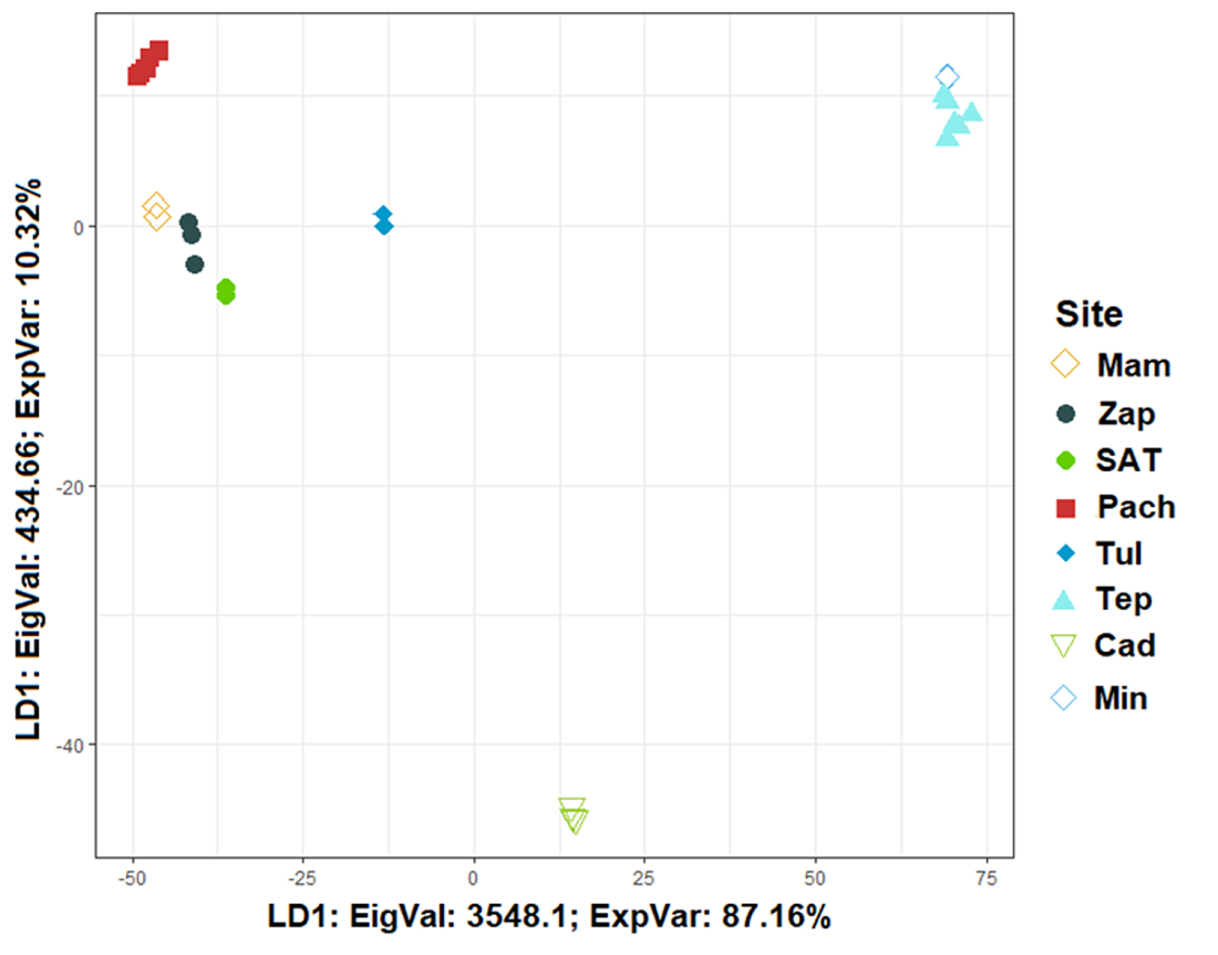
Figure 3 LDA plot at sites where disturbance analysis was carried out. Mam: Mambru. Zap: Zapotlan. SAT: San Agustin Tlaxiaca. Pach: Pachuca. Tul: Tulancingo. Tep: Tepelmeme. Cad: Cadereyta. Min: Mineral de Pozos.
The presence of roads frequently used by humans, agave plant carcasses, evidence of fire, and proximity to human activity centers are the attributes that had the most significant effect on the populations of Zap, Tul, and SAT. The Mam population was mainly affected by the distance to human activity centers and roads used by humans, but due to the population size, no impact of extraction was observed. Tep and Cad are located at opposite ends of the quadrant, with Tep having the most significant evidence of erosion. In contrast, Cad had the greatest presence of cattle excrement, roads used by cattle, and proximity to nuclei of human activity. There was no extraction on the sites not in Hidalgo. Pach had the largest completely modified area and the shortest distance to human settlements. However, the population size did not allow the effect of extraction to be perceptible. In Min, the most significant impact was due to proximity to population centers and the number of roads frequently used by humans, but there was no evidence of extraction.
The population with the highest disturbance index (di) was Cad, followed by Min and Pach. Tep and Tul had intermediate levels of disturbance. The sites with the lowest disturbance percentages were Zap and Mam. The Mam population had the most significant number of dry and overturned individuals associated with extraction activities, but is not representative in percentage respect total population, in contrast Pach had the highest percentage (Table 4).
Table 4 Affected area (di) expressed as a percentage. SD: standard deviation, %Ext: percentage of extraction.
| Population | di ± SD | %Ext |
|---|---|---|
| Mambru | 10.50 ± 7.32 | 10 |
| Zapotlan | 20.67 ± 20.12 | 1.6 |
| San Agustin Tlaxiaca | 29.08 ± 13.75 | 13.6 |
| Pachuca | 51.94 ± 0.83 | 35.3 |
| Tulancingo | 32.08 ± 14.97 | 9.3 |
| Tepelmeme | 45.83 ± 23.54 | 0 |
| Cadereyta | 81.89 ± 3.86 | 0 |
| Mineral de Pozos | 57.83 ± 23.81 | 0 |
Classification. The optimal number of size groups to explain the data structure is four, represented by k = 4 (Table 5). The correspondence analysis (CA) was significant (χ 2 = 497.17, d.f. = 21, P < 0.001, Eig. Dimension 1 = 0.15477, E.V. = 76.15 %, Eig. Dimension 2 = 0.045317, E.V. = 20.92 %). The analysis showed that seedlings are the dominant category in Mam, Zap, Pach, and SAT, while Tul, Tep, and Min consist mainly of juvenile individuals. The populations outside Hidalgo have the largest numbers of Adults 1 and 2, as shown in Figure 4.
Table 5 Average size of each of the categories generated from k = 4. These measurements are in centimeters. D1: Diameter 1, D2: Diameter 2. We did not find individuals with heights between 10 and 20 cm, so there is a gap between the seedling and juvenile categories.
| Category | Height | D1 | D2 |
|---|---|---|---|
| Seedlings | 4.68 ± 3.97 | 7.3 ± 5.41 | 5.96 ± 5.52 |
| Juveniles | 27.12 ± 7.36 | 34.67 ± 9.06 | 34.30 ± 10.08 |
| Adult 1 | 64.3 ± 18.22 | 78.3 ± 15.45 | 80.7 ± 21.09 |
| Adult 2 | 167.5 ± 3.53 | 205.5 ± 0.7 | 198 ± 2.82 |
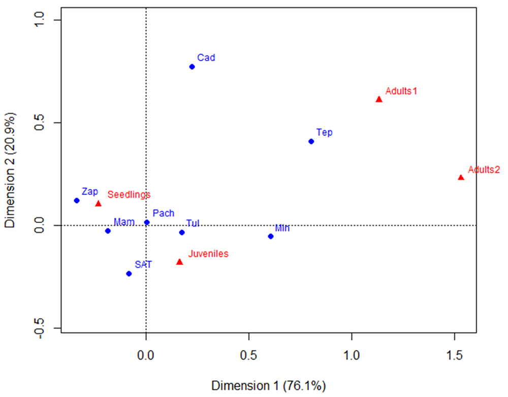
Figure 4 Correspondence analysis (CA) between size categories (letters in red) and populations (letters in blue). The explained variance (EV) is shown in parentheses. Mam: Mambru. Zap: Zapotlan. SAT: San Agustin Tlaxiaca. Pach: Pachuca. Tul: Tulancingo. Tep: Tepelmeme. Cad: Cadereyta. Min: Mineral de Pozos.
The populations show an aggregate spatial distribution in patches dominated by many seedlings (approximately 50 individuals per square meter). The frequency of individuals with a height between 10 and 20 centimeters is so low that they hardly appear in the categorization, we can see a “gap” in the size of seedlings to juveniles (3.97 to 27.12 cm) (Table 5, Figure 5).
Static life tables and survival curves. The eight populations of maguey have an average number of viable and non-viable seeds per fruit of 221.6 ± 27.46 SD and 201.66 ± 59.61 SD, respectively. On average, the peduncle (“quiote”) has 16 ± 4 panicles, and the branch has an average of 4.5 ± 2.75 panicle umbels (infructescences). Based on these data, the number of viable seeds per individual is 254,592 ± 7,630. The intrinsic rate of population growth calculated based on sexual reproduction shows that all the populations are decreasing, especially the Zap and Pach populations, which have the lowest λ, and both have extraction. The net reproductive rate (R0) is low in all populations, indicating that very few sexual offspring can reproduce. The average life expectancy (ex) is one category, which means only juvenile individuals are likely to become Adult 1. The SAT population does not show Adult 2 (sexual reproduction), so it is not possible to calculate demographic indicators (Table 6).
Table 6 Demographic indicators of population growth for sexual reproduction (by seeds) and asexual reproduction (by offshoots). R0: Net reproductive rate. TG: Generational time. r: Per capita population growth rate. λ: Intrinsic population growth rate. ex: Average life expectancy for all categories. SAT: San Agustin Tlaxiaca.
| Population | Sexual reproduction | Asexual reproduction | ||||||||
|---|---|---|---|---|---|---|---|---|---|---|
| R0 | TG | r | λ | ex | R0 | TG | r | λ | ex | |
| Mambru | 0.0000157 | 4 | -2.766 | 0.063 | 0.960 | 6.230 | 3 | 0.610 | 1.840 | 1.422 |
| Zapotlan | 0.0000038 | 4 | -3.120 | 0.044 | 1.160 | 0.076 | 3 | -0.855 | 0.425 | 1.520 |
| SAT | 0 | 0 | 0 | 0 | 0 | 0.076 | 3 | -0.855 | 0.425 | 1.494 |
| Pachuca | 0.0000038 | 4 | -3.120 | 0.044 | 1.210 | 0.076 | 3 | -0.855 | 0.425 | 1.598 |
| Tulancingo | 0.00003 | 4 | -2.600 | 0.074 | 1.290 | 0.307 | 3 | -0.393 | 0.675 | 1.895 |
| Tepelmeme | 0.0000228 | 4 | -2.672 | 0.069 | 1.410 | 6.230 | 3 | 0.610 | 1.840 | 1.983 |
| Cadereyta | 0.0000076 | 4 | -2.947 | 0.053 | 1.270 | 13 | 3 | 0.855 | 2.351 | 1.602 |
| Mineral de Pozos | 0.0001253 | 4 | -2.246 | 0.106 | 1.340 | 135.69 | 3 | 1.637 | 5.139 | 2.397 |
When we evaluate the demographics considering vegetative reproduction, we find that the intrinsic population growth rate (λ) exceeds unity in the Mamb (population with extraction) and the three populations outside Hidalgo, Tep, Cad, and Min. Compared to sexual reproduction, there was a significant increase in this parameter in the rest of the populations (χ > 250, P < 0.0001), but without exceeding unity, indicating a decrease in these populations. When analyzing the net reproductive rate via asexual reproduction (R0), we observe a significant increase in the same populations(χ = 165.1, P < 0.0001) (Mam, Tep, Cad, and Min), which increases vegetative progeny that will reach the Adult 1 and 2 categories. In all cases, the average life expectancy (ex) increases, but no significatively among sexual vs vegetative reproduction (χ = 1.67, P = 0.97), with the maximum transition seen in Min, where two categories will pass to their next life stage (Table 6). All populations have inverted “J” survival curves, with high mortality in the early stages (seeds and seedlings) and a slight recovery in the juvenile and adult ages (Figure 6).
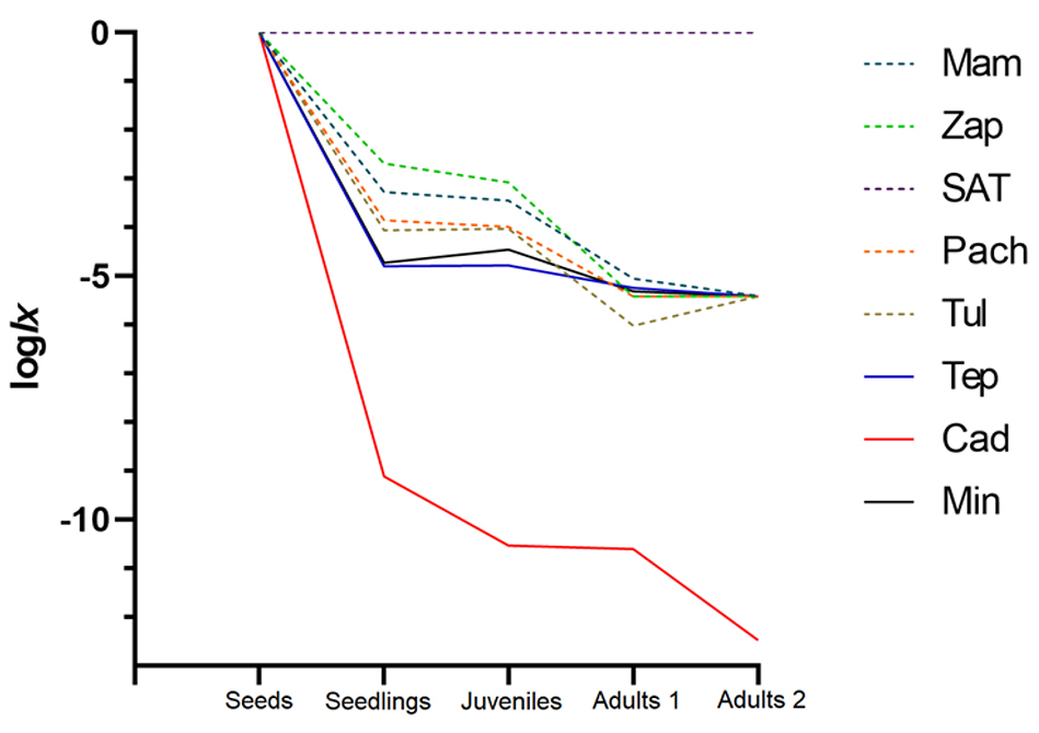
Figure 6 Type III survival curves (inverted J). Indicates a strong pattern of mortality in the first stages of life and slight recovery in subsequent stages. Mam: Mambru. Zap: Zapotlan. SAT: San Agustin Tlaxiaca. Pach: Pachuca. Tul: Tulancingo. Tep: Tepelmeme. Cad: Cadereyta. Min: Mineral de Pozos.
Correlation of disturbance vs demographics. The results of the Shapiro-Wilks test showed that some of the data being compared were not normal (for Ext, W = 0.145, P = 0.129, for di W = 0.064, P = 0.935, for λsexual W = 51.87, P = 0.005 and for λasexual W = 47.77, P = 0.004). There was a positive and significant Spearman correlation between the means of the paired perturbation between populations (di) and the difference in standardized growth rates obtained by asexual reproduction (ln((Δ𝜆)2) veg) (r = 0.411, P = 0.030, Figure 7). However, the latter does not correlate with extraction. Additionally, the difference between standardized population growth rates obtained sexually (ln(Δ𝜆)2sex) does not correlate either with disturbance (di) or extraction (Ext).
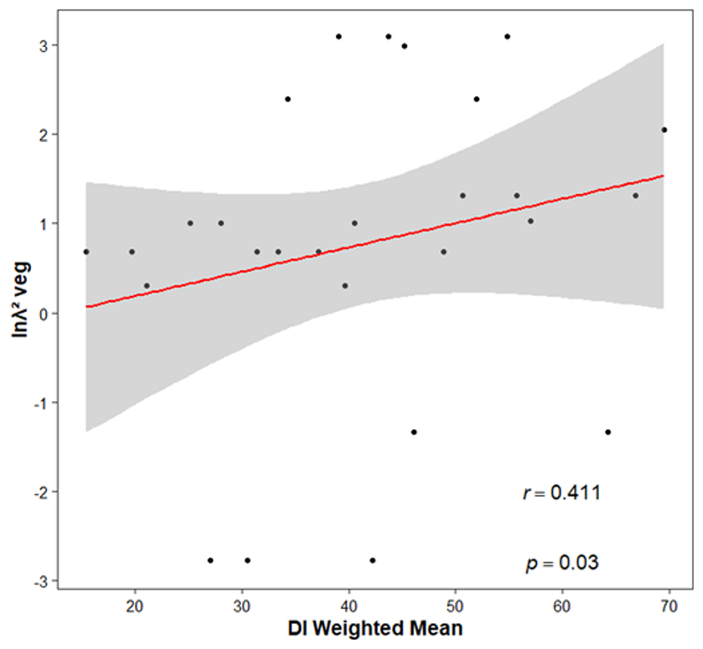
Figure 7 Spearman correlation with two of the weighted variables. The trend line and the 95% confidence interval are shown. The X axis represents the paired average between populations of the disturbed area (di) and the Y axis shows the natural logarithm of the finite population growth rate obtained through the vegetative data (λveg) squared.
Discussion
In Agave applanata populations, disturbance significantly impacts the population growth rate, but only when growth is obtained by asexual reproduction. Since juveniles have the highest production of offshoots, they are the most important category for the persistence of the species. Non-harvested populations have the highest population growth rates, with harvesting leading to a 57 % decrease in population size. However, data on disturbance show that moderate human disturbance can favor this species. It has been observed that moderate human disturbance can benefit this species if chinicuil is not collected.
It has been observed that disturbance is present in all the analyzed populations, but the extent of disturbance varies. It is important to note that no evidence of extraction exists in any population except for those in Hidalgo. However, it was precisely in those localities where livestock farming, and habitat deterioration showed the highest values. This indicates that human disturbance hurts multiple levels of organization (Cole & Landres 1996) with varying impacts depending on the age of the plants, as classified in this study by size categories. Cattle can reduce population density and hinder regeneration by biting and trampling plants in early stages, which results in poor regeneration and seedling establishment (Martin et al. 2011), as seen in Cadereyta.
Extraction of chinicuiles has had the most significant impact on the evaluated populations within Hidalgo. This is evident from the reduced number of adult plants and the absence of individuals between 10 and 20 cm in height (Table 5, Figure 4). According to Martínez-Ramos et al. (2016), anthropogenic disturbance can cause a homogeneous size structure, leading to a lower proportion of large plants. However, the results indicate that there is also a lack of plants that initiate the juvenile stage, suggesting that these are the ones being used to obtain the chinicuiles.
Population-level studies have shown that disturbance can have positive, negative, or neutral effects on density. In some cases, moderate disturbance levels can benefit certain species (Cervera et al. 2007, Portilla-Alonso & Martorell 2011, Martorell et al. 2012, Arias-Medellín et al. 2014). Agaves are known for their resilience to drought conditions, hot climates, and sun exposure (Davis et al. 2021). This explains why Agave applanata populations outside of Hidalgo have a higher density and better size structure, even with high levels of disturbance. Essentially, these populations are resilient and can thrive with moderate disturbance if chinicuil extraction does not occur.
Extraction. In 2017, it was discovered that chinicuiles inhabit not only A. salmiana but also A. applanata (Llanderal-Cázarez et al. 2017). However, producing chinicuiles from A. salmiana requires many maguey plants. To obtain one kilo of larvae, 54 magueys are needed. Up to 5.35 tons are produced, translating into approximately 20,000 plants per season (Briones-Santoyo et al. 2022, Montoya 2023). To calculate the amount of chinicuiles produced from A. applanata, we need to know the average weight of a larva and the number of worms present in each maguey. This information will allow us to estimate the number of plants needed to obtain one kilo of chinicuiles and so help us determine how many magueys are used in the region each season. We can also infer the approximate number of plants used by counting the number of corpses of maguey plants observed.
While many maguey plant carcasses exist in Hidalgo, the extraction percentage is not as high because it depends on the area analyzed. For example, in Mam and Zap, the extraction percentage is only around 10 % of the population due to the difficulty of harvesting chinicuiles on the slope, but the number is highest in the entirely analyzed sites (100 corpses). In contrast, the smaller area in Pach, with fewer plant carcasses, represents a high extraction percentage.
It is worth noting that chinicuil extraction is not occurring in areas outside Hidalgo, indicating that this activity is limited to specific regions. In Oaxaca, chinicuil is only harvested from mezcal agaves, which does not significantly impact the population of A. applanata (Martínez-Jiménez et al. 2019).
It has been suggested that the decline of the moth in the country during the last 15 years may be due to factors such as overexploitation of the larvae, changes in land use, deforestation, erosion, and changes in average annual rainfall levels. This decline is thought to be why the chinicuil attacks any available wild agave, even seeking alternative hosts other than Agave, such as Wigandia, Croton, Solanum, Mentzelia, Brickellia, Lippia, and Cordia (Chagoya-Lizama 2008). This behavior could lead to potential phytosanitary problems that should be considered in future studies.
Hidalgo’s government agencies have proposed a law to care for maguey and its derivatives. Sharing the information generated in studies such as this one is crucial, as there are no regulations for using and marketing this product. Understanding the actors’ social and economic situation is necessary for understanding the reasons behind their good or bad practices (Pijoan 2001, Ramos-Elorduy 2006, Ramos-Elorduy et al. 2006).
Static life tables and survival curves. The study found that there has been a decrease in the population of A. applanata in all regions when only fecundity based on sexual reproduction is considered. However, this is common in species with low recruitment rates and type III survival curves, where there is almost no movement to juvenile stages. These characteristics are typical of long-lived plants (Picó et al. 2008). Therefore, this approach indicates that all populations behave similarly with respect to generation time, life expectancy, and population growth rate, regardless of their status. In other words, static life tables that focus on sexual reproduction describe the species, without identifying specific environmental factors or monitoring the impact of chinicuil extraction on A. applanata over time.
In contrast, clonal growth results in the emergence of new individuals that can become independent if they survive separation. These offspring undergo almost all life cycle transitions except for the initial stages (Harper 1977, Klimeš et al. 1997). This means that recruitment increases without requiring seed mediation and can derive from both juveniles and adults. Moreover, there is no need to record a population drop during the seedling-to-seedling stasis or seedling-to-juvenile transition because the connection with the mother ensures longer survival. As a result, in the life tables obtained from asexual reproduction, an increase in λ was observed in all populations. However, it reached values greater than unity only in sites outside Hidalgo and Mam, implying a population reduction between 32.5 and 57.5 % in Zap, SAT, Pach, and Tul. Although it is less drastic than the population reduction calculated by the tables based on sexual reproduction, it is still significant. The most plausible explanation for such a reduction is only extraction, proportional to population size.
While clonal reproduction has its demographic benefits, the lack of sexual recombination can lead to inbreeding depression. However, in the case of agaves, it does not necessarily result in extinction. Both sexual and asexual processes offer distinct evolutionary pathways. Sexual reproduction accumulates new genetic diversity, while asexual reproduction perpetuates successful clonal variants with minimal somatic mutation load and lower energy expenditure (Ellstrand & Roose 1987, Gross et al. 2012, Jarni et al. 2015, Cruzan et al. 2022). A. fourcroydes, for instance, generates and transmits new somatic genetic variation mainly through asexual reproduction, resulting in stable and growing populations (Infante et al. 2003).
The survival curves for the Hidalgo sites have steeper slopes during the transition from juvenile to Adult 1, the most menaced transition for population persistence. We did not consider the seed-to-seedling drop since it is customary in long-lived plants (Octavio-Aguilar et al. 2008). However, eliminating the juvenile category threatens local extinction without any recovery time, as the annual collection exceeds the transition and recruitment period of this species.
Finally, it is recommended to use matrix projection models (MMP) or integral projection models (IPM) to project population dynamics accurately. These models allow for both prospective and retrospective analyses to determine which demographic categories and parameters are more vulnerable and which contribute more to the growth rate of the population (λ) (Doak et al. 2021).
Correlation of variables. The results imply that the greater the average disturbed area, the greater the difference between the population growth rate calculated from vegetative reproduction and from sexual reproduction. In other words, disturbance promotes clonality. This is observed in several species of agricultural importance whose management (clearing, pruning, partial harvesting, among others) favors the recovery of plants from vegetative growth, which is beneficial for the recovery of degraded areas (de la Fuente & Suárez 2008, Cornejo-Badillo 2018). On the other hand, disturbance can increase spatial aggregation in early categories and favor population growth and fecundity (Ayerde-Lozada & López-Mata 2006), but only when certain environmental aspects eliminate competition such as the opening of clearings in species with tolerance to direct sun exposure.
Magueys are known for their ability to tolerate drought and solar radiation, and their resilience in stressful conditions (Davis et al. 2021). Therefore, disturbance effects are not always adverse, and it is essential to distinguish the type of modification being evaluated, mainly because the impact of extraction is lessened when other anthropic factors come into play, such as distance from human activity and livestock. Similarly, population size is a limiting factor affecting the impact of extraction. It is often overestimated in small areas and underestimated in larger areas, specifically in the Mambru.
The population growth rate obtained from asexual reproduction is promoted by the disturbance associated with cattle ranching, environmental modification, and proximity to human activity centers. However, the collection of chinicuiles in Hidalgo reduces this rate, mainly affecting juveniles smaller than 20 cm. Therefore, it is recommended to focus on management by cultivation in nurseries and reintroducing organisms of this size.

