


 texto en
  Inglés (pdf)
 Artículo en XML
 Referencias del artículo
 Enviar artículo por email
 Citado por SciELO
  Similares en
SciELO
Similares en
SciELO 
 Permalink
Introduction
Drought is a prolonged dry period, compared with the historical precipitation, that can have an impact on the hydrological balance, and cause social and environmental problems. Mexico has been affected by severe droughts in recent years. Dobler-Morales and Bocco (2021) point out that the 2011-2012 drought is considered an extreme event for its severity and extension, as it covered 70 % of the country. In addition, authors claim that Mexico’s population is highly vulnerable to drought effects, especially the crop farmers highly dependent on rainfall, but also marginalized urban population with low access to water infrastructure. After such extreme event, the Mexican government implemented the “National Program Against Drought” which includes a preventive approach that seeks to monitor and forecast drought conditions (Arreguín-Cortés et al., 2016). The National Water Service observes conditions of shortage or excess of precipitation with the Mexican Drought Monitor (MDM), which is constructed by several indices in layers blended through a Geographic Information System (Lobato-Sánchez, 2016). The MDM is an online tool that displays current and historical drought conditions in the country at biweekly intervals (Servicio Meteorológico Nacional [SMN], 2023).
For drought monitoring, good quality precipitation data is required (Lobato-Sánchez, 2016); however, as in many countries of the world, Mexican historical meteorological records present several problems. For instance, the study of Livneh et al. (2015) noted a sharp decline of the Mexican station density since 2000, particularly after 2006. In addition, the authors identified northern Mexico as an area of low station density. To fill the gap of reliable meteorological observations, the ability of precipitation products (i.e. interpolated observations and satellite estimations) to perform drought monitoring (in different countries and climatic type zones) have been evaluated.
Hinge et al. (2021) conducted a meta-analysis of these studies, and authors identified two main datasets in literature: CHIRPS (Climate Hazards Group infrared precipitation with station data) and PERSIANN-CDR (Precipitation Estimation from Remotely Sensed Information Using Artificial Neural Networks - Climate Data Record). Such datasets are preferred due to their long-term data record. The studies used the standard precipitation index (SPI) to estimate meteorological drought, and authors identified the dependence of performance on factors such as the climatic type and the length of the data record. They also suggest that future work should focus on identifying the best climatological condition under which each dataset performs best.
Rivera et al. (2019) evaluated the ability of the CHIRPS dataset to identified drought periods compared with rain gauge data in Argentina. The SPI was computed for several timescales (1, 3, and 6 moths) for the period 1987-2016. The evaluation was based in the correlation coefficient and the mean absolute error. Results show that, in arid and semiarid regions, the precipitation dataset adequately reproduces the frequency of wet and dry periods on time scales larger than one month.
The ability of the CHIRPS dataset to detect droughts was also evaluated in the Mekong River for the 1981-2016 period (Guo et al., 2017). The evaluation was conducted in terms of correlation, several error metrics, and droughts indicators of occurrence, intensity and area. Results show a better performance of the dataset to reproduce the 3-month SPI than the 12-month SPI; in addition, the drought events were well detected in terms of temporal evolution, occurrence and distribution.
Zambrano et al. (2017) compared two precipitation datasets, CHIRPS and PERSIANN-CDR, with in situ observations in the evaluation of the SPI at several time scales (1, 3 and 6 moths) for different climatic regions in Chile. The authors found, based in RMSE and correlation, that better results on SPI were observed in regions with a superior fit in the precipitation, and argue that the precipitation products should be calibrated to adjust for the overestimation and underestimation.
Most of the studies that evaluates CHIRPS and PERSIANN-CDR for drought monitoring were conducted in Asian countries, and few research in this topic has been carried out in Mexico (Hinge et al., 2021). de Jesús et al. (2016) evaluated the Tropical Multi-Precipitation Analysis (TMPA 3B42) product for its ability to reproduce the SPI computed with a 15-year record of observations from three meteorological stations located in different climatic regions. The results show a low correlation in the SPI times series, and the authors identified the short length of the record and the poor agreement in the rainfall estimates as the main cause of poor performance. However, authors claim that the use of the selected dataset can be used to detect severe drought periods.
Several studies have reported an increase in the severity and frequency of drought events worldwide (Spinoni et al., 2014). Stahle et al. (2009), argue that climate experiments indicate that Mexico will experience dryer conditions in the 21st century due to global warming, with the potential convergence of natural and anthropogenic droughts. In this regard, the study of Spinoni et al. (2020) evaluated the changes in droughts indicators based on climate simulations from the Coordinated Regional Climate Downscaling Experiment (CORDEX) for the period 2071-2100 versus the period 1981-2010. The results identified red spots of future meteorological droughts, that is, areas that show a robust increase in drought frequency and severity, including coastal North America, most of Mexico and northern Central America.
The use of climate simulations from Global Climate Models (GMC) should be downscaled and bias corrected for their use in shorter scales (Velázquez-Zapata, 2019). Hinge et al. (2021) claim that in the estimation of historical SPI, bias correction methods (such as quantile mapping) should be applied to precipitation products before calculating SPI to improve its performance. Considering the above, the objectives of the present study were to evaluate three high-resolution precipitation datasets to capture the annual cycle and trend, and to reproduce SPI values and drought indicators from seven meteorological stations located in central Mexico. Also, to determine the influence of the precipitation products used as a reference point for the statistical correction of climate simulations in the evaluation of precipitation change between the reference period and the future, and the estimation of drought indicators for the period 2040-2100.
The study area is the Low Panuco River, which was selected because this region presents various climatic types. The Panuco River Basin is one of the most important basins in Mexico for its extension (96 986 km2) and runoff (20 329 hm3∙year-1) (Pedrozo-Acuña et al., 2015). The basin is divided in two main regions: the Moctezuma River Basin and the Tampaon River Basin (del Ángel-González & Domínguez-Mora, 2015). The first originates from the Tula River (State of Hidalgo) and flows from Mexico City to the northeast. The second has its headwater in the Santa María River, and it flows from west to east in the states of Guanajuato and San Luis Potosí. The confluence of the Moctezuma and the Tampaon River takes the name of Panuco River. A few kilometers before the river discharges into the Gulf of Mexico, the Panuco River receives the contribution of the Tamesi River (state of Tamaulipas) from northwest.
Materials and methods
Study area and precipitation datasets
Figure 1 shows the Low Panuco River Basin. The Panuco River basin area has a variety of climatic regions, as a result of the topographic variation in the Sierra Madre Oriental mountain chain (Velázquez-Zapata & Troin, 2020). The western region has an arid climate, the central region has temperate climate, and the eastern region has a tropical climate (Peel et al., 2007). Table 1 shows the meteorological stations, the type of climate and the average annual precipitation in the period 1983-2013, which ranges from 387 mm in the arid region to 2 673 mm in the tropical region.
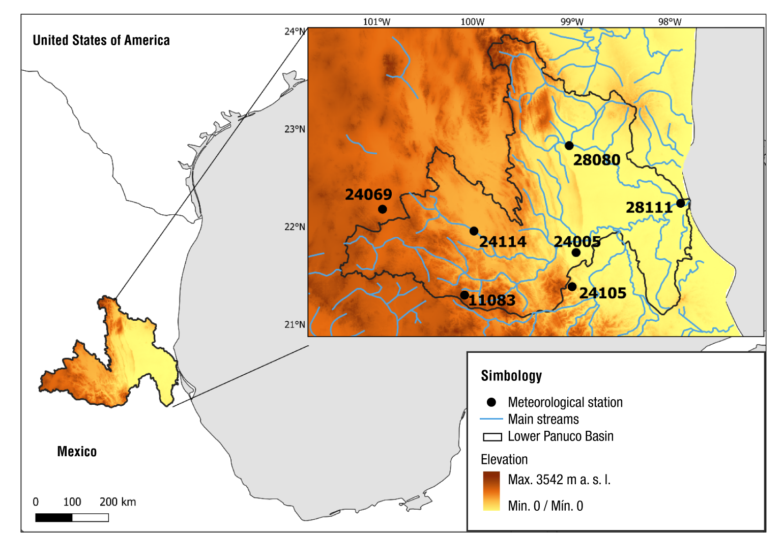
Table 1 Meteorological stations and mean annual precipitation for the period 1983-2013 in the Panuco River basin.
| ID | Name | Climate type | Elevation (m) | Mean annual precipitation (mm) |
|---|---|---|---|---|
| 24069 | San Luis Potosí | BsK | 1 870 | 387 |
| 11083 | Xichu | CwA | 1 318 | 558 |
| 24114 | Rioverde | CwA | 991 | 500 |
| 24105 | Xilitla | Af | 676 | 2 673 |
| 24005 | Ballesmi | Af | 45 | 1 513 |
| 28080 | Rio Frio | Aw | 60 | 1 058 |
| 28111 | Tampico | Aw | 3 | 1 157 |
Meteorological data were obtained from four datasets: meteorological stations and three high resolution datasets. The observed monthly precipitation was taken from seven stations of the SMN, hereinafter called SMN data. Table 2 shows the selected high-resolution datasets: NOAA data were retrieved from the database proposed by Livneh et al. (2015) which consists of observed daily precipitation gridded to a 1/16°. For Mexico, precipitation data were provided by the SMN, and the methodology for developing the data includes orthographic precipitation adjustment. Funk et al. (2015) proposed the CHIRPS data. The methodology to create the precipitation estimates combines satellite precipitation measurements and ground station data to produce precipitation time series and perform trend analysis and seasonal drought monitoring with 0.05° resolution on a monthly time interval.
Table 2 Selected high-resolution precipitation datasets.
PERSIANN-CDR data were retrieved on a monthly time interval (Nguyen et al., 2018). This dataset was built with an artificial neural network methodology based on satellite estimates and adjusted for precipitation climatology. All datasets were obtained for the period 1983-2013, and were analyzed on a monthly interval NOAA data were aggregated monthly; therefore, all datasets in this study were analyzed on a monthly interval. To compare the precipitation gridded data with observations, the closest gridded point to each weather station (with Euclidean distance) was selected and considered as a proxy station (Ghorbanian et al., 2022).
In addition, climate simulations were retrieved from the second generation Canadian Earth System Model (Arora et al., 2011) under the Representative Concentration Pathway rcp8.5, which considers a scenario of high greenhouse emission in the next decades. The five members ensemble precipitation simulations were obtained for the historical period 1983-2013 and the future period 2040-2100. Precipitation simulations were downscaled and bias-corrected with the method proposed by Mpelasoka and Chiew (2009). This method establishes, in a first step, a relationship (correction factors) between the simulated and the observed precipitation in the historical period (ref) at different percentiles (Equation 1). In a second step, correction factors were applied to precipitation outputs in future periods (fut,Equation 2):
where P corr is the bias-corrected precipitation. The indexes correspond to percentile (q), month (m), raw climate simulations (sim) and observations (obs) or another meteorological dataset used in this study. The bias correction method is applied on a monthly basis, and it was carried out for each meteorological (and proxy) station, so for each one of them, five climate simulations were obtained, that allowed to evaluate the natural variability of the climate (Muerth et al., 2013).
Standard precipitation index and evaluation methods
The SPI analyses the wet and dry cycles as an indicator of drought periods and is based on the evaluation of the probability of precipitation at different timescales (McKee et al, 1993). The SPI computation requires precipitation time-series, which are fitted to a probability distribution, so the mean SPI is zero (Edwards & McKee, 1997). Therefore, positive (negative) SPI values indicate greater (less) values than the median precipitation (World Meteorological Organization [WMO], 2012). The classification of wet and dry periods, based on the SPI, is shown in Table 3.
Table 3 Standard precipitation index values.
| Values | Classification |
|---|---|
| 2.0 and more | Extremely wet |
| 1.5 to 1.99 | Very wet |
| 1.0 to 1.49 | Moderately wet |
| -0.99 to 0.99 | Near normal |
| -1.0 to -1.49 | Moderately dry |
| -1.5 to -1.99 | Severely dry |
| -2.0 and less | Extremely dry |
Source: World Meteorological Organization (WMO, 2012).
In this work, the SPI was computed with the 12-month accumulation period. The use of SPI-12 reflects long-term precipitation anomalies that affect groundwater, streamflow and reservoir storage (WMO, 2012). The drought periods were evaluated with SPI values obtained with the precipitation datasets described in Table 2 based in the methodology described by Spinoni et al. (2020). These authors who define the start of a drought event when the SPI value falls below -1, for at least two consecutive months, and it ends when the SPI value turns positive. The authors also define the following indicators:
Evaluation metrics
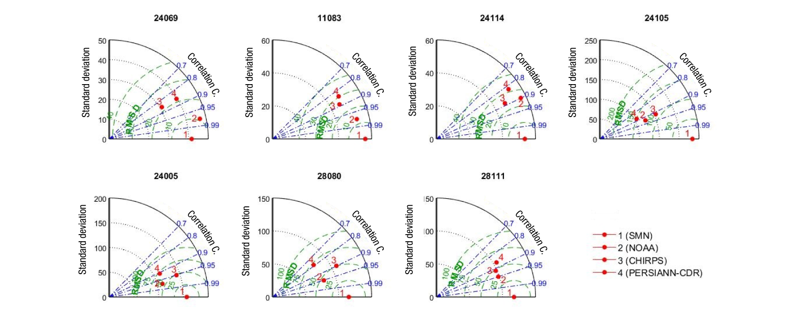
The gridded precipitation was compared with the observed precipitation in terms of their correlation, the root-mean-square difference, and their standard deviations through the Taylor Diagram that summarizes the degree of correspondence between the two fields (Taylor, 2001).
The correlation coefficient R, between the variables x and y which are defined in N discrete points is calculated as:
where
RMSE approaches to zero when the fields are more alike. The Taylor diagram uses the relationship between the statistical quantities R, RMSE and σ x , σ y to represent the association between the variables with a single point.
The precipitation datasets were also compared in terms of variability using the coefficient of variance (CV) which is defined as the ratio of the standard deviation to the mean. The trend in the datasets was evaluated and compared with the Sens’s slope, which estimates the slope of the trend using the following equation:
where x j , x k are the values of the variable in the given years j and k (j > k). A positive (negative) value of β indicates an increasing (decreasing) trend in the time series (Kubiak-Wójcicka et al., 2021)
Finally, the gridded datasets were compared to the observations in terms of their ability to detect the occurrence of the wet and dry periods. The scores are based in the comparison of forecasted events and observed events (Table 4).
Table 4 Contingency table.
| Forecast | Event observed | |
|---|---|---|
| Yes | No | |
| Yes | Hit (a) | False alarm (b) |
| No | Miss (c) | Correct not event (d) |
Source: Ghelli (2009).
The categorical scores are the probability of detection (POD), the false alarm ratio (FAR) and the critical success index (CSI) computed with the following equations:
The POD shows the ability of the precipitation dataset to capture the SPI value computed with observations (perfect score = 1), FAR indicates the incorrect detection of the SPI value (perfect score = 0) and CSI is the overall fraction of SPI correctly detected (perfect score = 1, no skill = 0) (Ghorbanian et al., 2022; Ghelli, 2009). A SPI value obtained with a given dataset (forecasted) is considered detected if it falls in the same range of the SPI obtained with observed precipitation (according with table 3).
Results and discussion
The observed precipitation records are homogeneous, based on the Helmert test (Campos-Aranda, 1988). The selected gridded precipitation datasets were compared with observations on their ability to capture the annual cycle for the period 1983-2013. Figure 2a shows the variability in the observed precipitation among the meteorological stations as they have different climate types. In general, the annual cycle has two peaks in July and September, with a decrease in August that corresponds to the midsummer drought (MSD). As mentioned by Magaña et al. (1999), the MSD does not correspond to a real period of drought but rather to a decrease in the amount of rain. The gridded precipitation datasets (Figure 2b to 2d) also capture the MSD and have a good overall representation of the annual cycle.
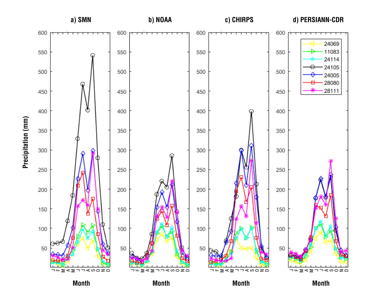
Figure 2 Annual cycle of precipitation obtained with the selected datasets for the period 1983-2013.
Precipitation varies between models and stations. Proxy stations located in dry and temperate climates (stations 24069, 11083 and 24114) have a good representation of the amount of precipitation. The differences, with respect to the NMS data, are 3 and -5 % for NOAA and CHIRPS data, respectively. The difference evaluated with the PERSIANN-CDR data is about 22 %. The proxy stations located in the humid tropical climate type (24005, 28080 and 28111) show an underestimation of precipitation of approximately -24, -16 and -27 %, with NOAA, CHIRPS and PERSIANN-CDR data, respectively. The largest underestimation is observed in the humid mountainous climate type (station 24105), with values ranging from -50 to -60 %.
Figure 3 shows the Taylor Diagram that evidences the statistical relationship between the precipitation datasets. In general, NOAA data presents the best correlation with SMN data (0.94). CHIRPS data and PERSIANN-CDR data present correlation coefficients of the order of 0.9 and 0.85, respectively. The standard deviation is well represented at stations 24069, 11083 and 24114. For example, at station 24069 the standard deviation obtained with observations is 41.6 mm, and the value of the resulting statistic with NOAA data, CHIRPS data and PERSIANN-CDR data is 46.8, 31.0 and 39.4 mm respectively. On the other hand, the difference is greater in stations with a humid climate type. For instance, at station 24105, the value of the standard deviation is 233.54 mm, while the statistic is 124, 154 and 105 mm for NOAA data, CHIRPS data and PERSIANN-CDR data respectively. This result indicates the lower variability of the selected precipitation datasets compared to observations. Regarding the RMSE, in general, PERSIANN-CDR data shows the largest errors and NOAA data the smaller ones.
The differences in the variability of the data can also be seen in Figure 4a which shows the CV, so SMN data has the higher variability compared with the other datasets. In addition, Figure 4b shows the trend of the time series with the Sen’s slope (calculated on an annual basis). In general, SMN data shows no trend with a median value of 0.2 %, while NOAA data, CHIRPS data and PERSIANN-CDR data have median values of the Sen’s slope of -5.5, -2.3 and -4.6 %, respectively. The greater decrease trend was reported in station 24105 with SMN data (-23 %) and NOAA data (-19 %).
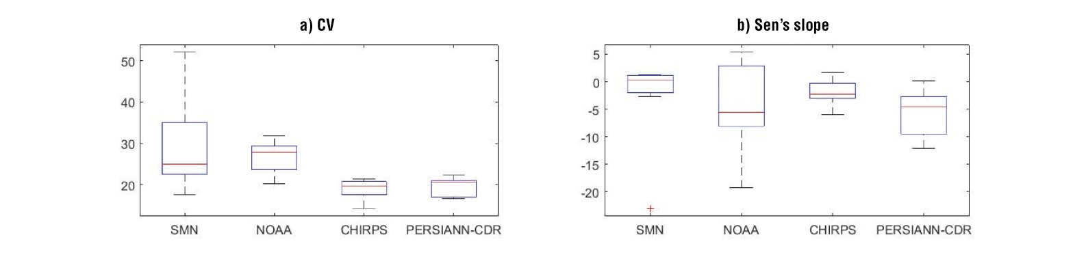
Figure 4 Coefficient of variance and Sen’s slope. Each boxplot is constructed with the results from the seven meteorological (or proxy) stations, and each box ranges from 0.25th to 0.75th percentile, with the center line being the median.
The SPI-12 computed with the four datasets and the frequency of the results are shown in Figure 5 and Figure 6 for station 24069 and 24005 respectively. These Figures show that the observed dry and wet periods (based on SMN data) occur at different moments among the stations. For instance, the wet period in 1994 at station 24005 is a normal period at station 24069, and the observed dry periods in 2000-2001 and 2011-2013 at station 24069 are normal periods at station 24005.
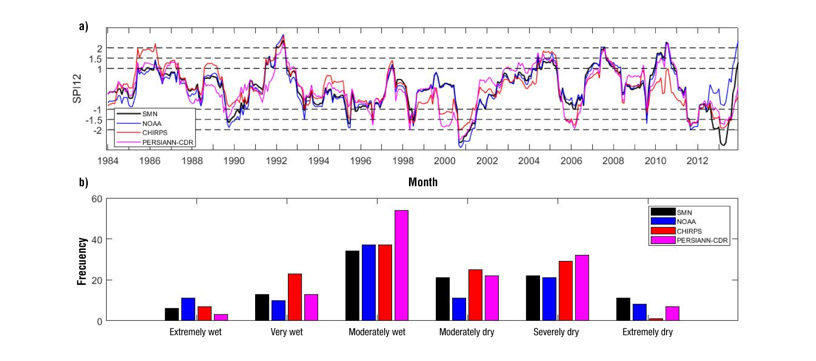
Figure 5 Standardized 12-month precipitation index (SPI-12) (a) and frequency (b) of results for station 24069.
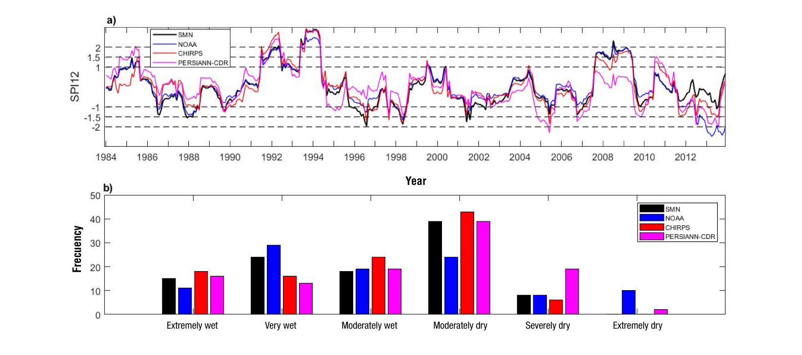
Figure 6 Standardized 12-month precipitation index (SPI-12) (a) and frequency (b) of results for station 24005.
In general, Figure 5a shows a good agreement between the values obtained with the observations and the precipitation data, but some differences lead to a different classification. The observations classify the 1985-1986 period as moderately wet, while the CHIRPS data identify this period as extremely wet. Similarly, the observations define the 2006 period as near normal, while the SPI-12 obtained with NOAA and CHIRPS data classifies this year as severely dry. In general, NOAA data show good agreement with the SMN data, except for the period 2012 and 2013. The difference in SPI evaluated with the datasets is also evident in the frequency of events (Figure 5b). In this figure, a high frequency of very wet events can be observed with CHIRPS, and moderately wet with PERSIANN-CDR. On the other hand, the results show a low frequency of moderately dry events with NOAA, and extremely dry events with CHIRPS.
Table 5 shows the correlation coefficient calculated with SPI-12 between the observations (SMN data) and the other data sets. At station 24069, the correlation coefficients are 0.92, 0.83 and 0.84, for NOAA, CHIRPS and PERSIANN-CDR data, respectively. These results agree with those presented in the literature for SPI-12. Guo et al. (2017) report an R of 0.85 with CHIRPS, while Wei et al. (2019) show values of 0.84 and 0.95, for CHIRPS and PERSIANN-CDR, respectively, and Alijanian et al. (2019) obtained an R of 0.35 with PERSIANN-CDR. Hinge et al. (2021) mention that the performance of precipitation products in SPI evaluation depends, to a large extent, on the climatology of the site.
Table 5 Correlation coefficients between Sistema Meteorológico Nacional (SMN) data and the other datasets.
| Station | NOAA | CHIRPS | PERSIANN-CDR |
|---|---|---|---|
| 24069 | 0.92 | 0.83 | 0.85 |
| 11083 | 0.98 | 0.62 | 0.52 |
| 24114 | 0.80 | 0.83 | 0.77 |
| 24105 | 0.69 | 0.82 | 0.77 |
| 24005 | 0.89 | 0.92 | 0.77 |
| 28080 | 0.94 | 0.77 | 0.34 |
Similarly, Figure 6a shows the differences in the computation of wet and dry periods with the selected datasets for station 24005. For instance, the 1996-1997 dry period identified with observations is not well captured with CHIRPS data nor PERSIANN-CDR data, as these datasets identify this period as near normal. Another case is the 2012-2013 normal period which is reported as a dry period with the other datasets. Similarly, the dry period between 2007 and 2009 is not reported with PERSIANN-CDR data. The correlation coefficients for the SPI values obtained between SMN data and the other datasets are 0.89, 0.92 and 0.77 for NOAA data, CHIRPS data and PERSIANN-CDR data respectively. The differences in the frequency of the events are shown in Figure 6b. For example, NOAA data shows a high frequency of very wet events and low frequency of moderately dry events. On the other hand, extremely dry events were not reported with SMN data, but with NOAA data and PERSIANN-CDR data.
Figure 7 shows the frequency of wet and dry events evaluated for the meteorological and proxy stations. For extremely wet events (Figure 7a), the median values of the boxplots are close to that obtained with SMN data; however, NOAA data shows less variability. The median of the very wet events (Figure 7b) is similar among the datasets, but the moderately wet events (Figure 7c) identified with PERSIANN-CDR data are low in number (median value of 24) compared to the other datasets (33-35 events).
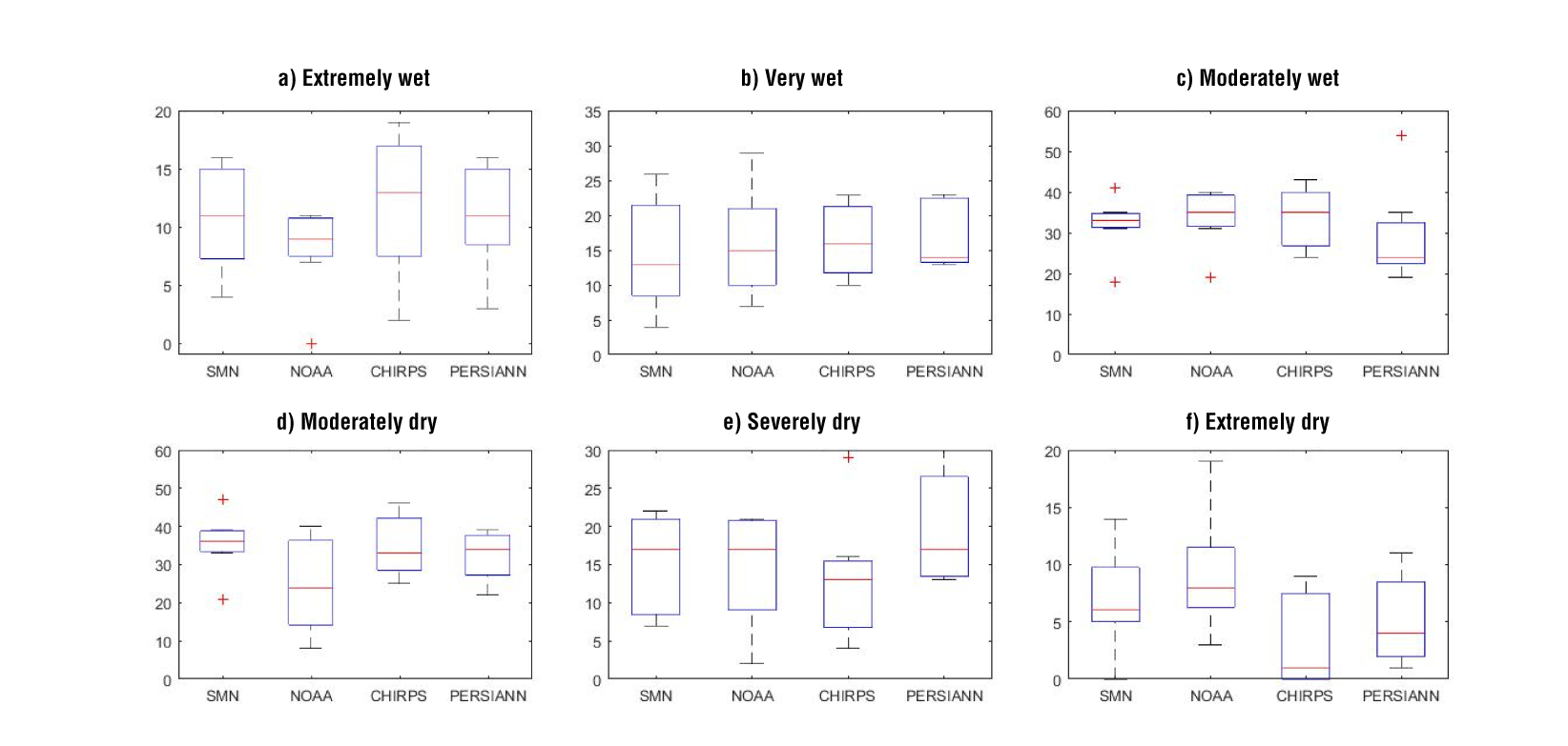
Figure 7 Frequencies of wet (upper panels) and dry (down panels) events computed with the selected datasets. Each boxplot is constructed with the results for the seven meteorological (or proxy) stations.
For moderately wet and moderately dry events, gridded precipitation datasets show greater variability compared with observations (SMN data). In the latter case, NOAA data shows a smaller median value (24 events) than the other datasets (about 34 events). For severely dry events (Figure 7e), CHIRPS data presents a lower median value than SMN data. Finally, CHIRPS data and PERSIANN-CDR data underestimate extremely dry events (Figure 7f). In other words, the selected gridded precipitation datasets would not correctly reflect the dry conditions in the analyzed period, despite the good correlation coefficient (Table 5).
Figure 8 shows the ability of the datasets to detect the occurrence of wet and dry events with the scores presented in Equations 6 to 8. In this figure, dry events include the three categories: moderately, severely and extremely dry, and similarly for wet events. In general, this figure shows that NOAA data performs best, compared with CHIRPS data and PERSIANN-CDR data. For instance, for wet events, the median value of POD is 0.61, 0.26 and 0.19 for NOAA data, CHIRPS data and PERSIANN-CDR data, respectively. Similarly, for dry events the median POD value is 0.43, 0.21 and 0.14 for NOAA data, CHIRPS data and PERSIANN-CDR data respectively. The median value of the FAR score is higher for CHIRPS data and PERSIANN-CDR data than for NOAA data in both wet and dry events; however, NOAA data presents a better result in wet events (0.3) than in dry events (0.4). The worst result in FAR was obtained with PERSIANN-CDR data, so the median value of the score is 0.75 and 0.87 for wet and dry events respectively. The CSI score shows similar results, so NOAA data has the best overall performance to correctly detect a given event (i.e., relative to SMN data), especially in the wet period.
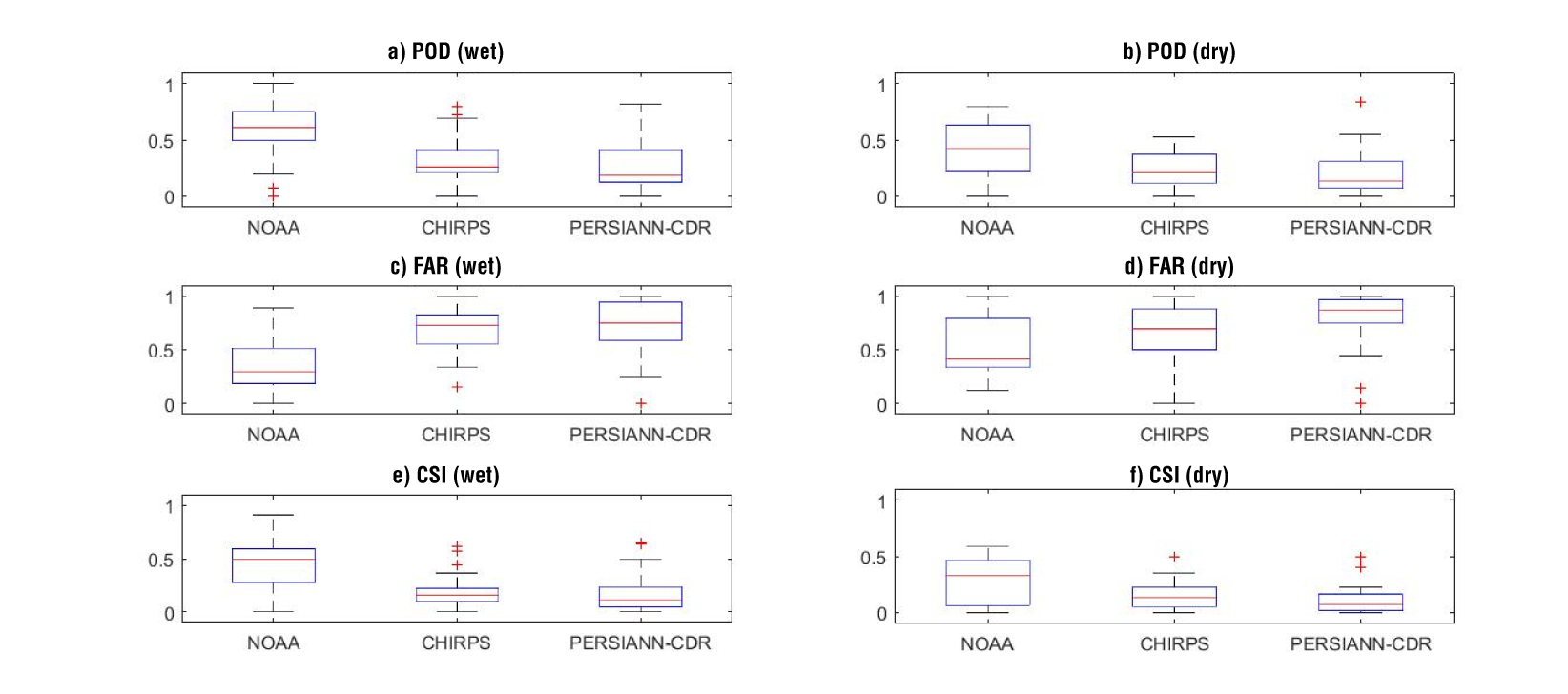
Figure 8 Results of the Probability of Detection (POD), the False Alarm Ratio (FAR) and the Critical Success Index (CSI) for wet events (center panels) and dry events (right panels). Each boxplot is calculated with 21 values corresponding to the results of seven meteorological (or proxy) stations and the three types of wet (or dry) events according to Table 3.
Figure 9 shows the boxplots corresponding to the drought indicators in the period 1983-2013. From this figure, we can see that the median of the drought frequency indicator is very similar among the selected precipitation datasets (five to six events), except for CHIRPS data, that presents seven events. In addition, NOAA data shows a larger range of events (from one to eight). The median value of the mean drought severity ranges from 13 (CHIRPS data) to 16 months (NOAA data), and the maximum drought severity ranges from 26 (NOAA data) to 29 months (CHIRPS data). Overall, all datasets show similar median indicators, but the range of the results is different among them, especially in the case of PERSIANN-CDR data which has the least variability in the severity indicators, that is, this dataset would underestimate or overestimate the number of months that a given drought would last. Similar results are reported in literature. For instance, Alijanian et al. (2019) observed, in a study conducted in Iran, differences in the number of total months with drought conditions, and in the maximum duration of the drought between PERSIANN-CDR and the gauge stations.
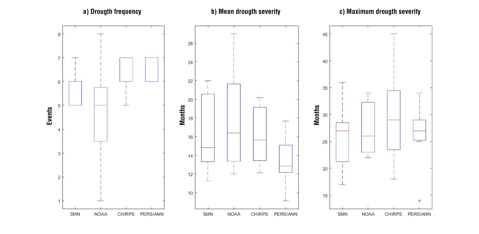
Figure 9 Drought indicators in the period 1983-2013. Each boxplot is built with the results of the seven meteorological (or proxy) stations.
Figures 10 and 11 show the annual cycles of precipitation in historical and future periods and the projected changes in precipitation computed for station 24069 and station 24005 respectively. The climate simulations were bias corrected by using each precipitation dataset as a benchmark. From this figure, we can see that, in the historical period, the annual cycle is well represented in both stations, but not with CHIRPS data in station 24069. In addition, some differences can be noted in the amount of precipitation (relative to SMN data); for example, at station 24069, NOAA data and CHIRPS data show a higher precipitation than SMN data, while at station 24005 the opposite occurs.
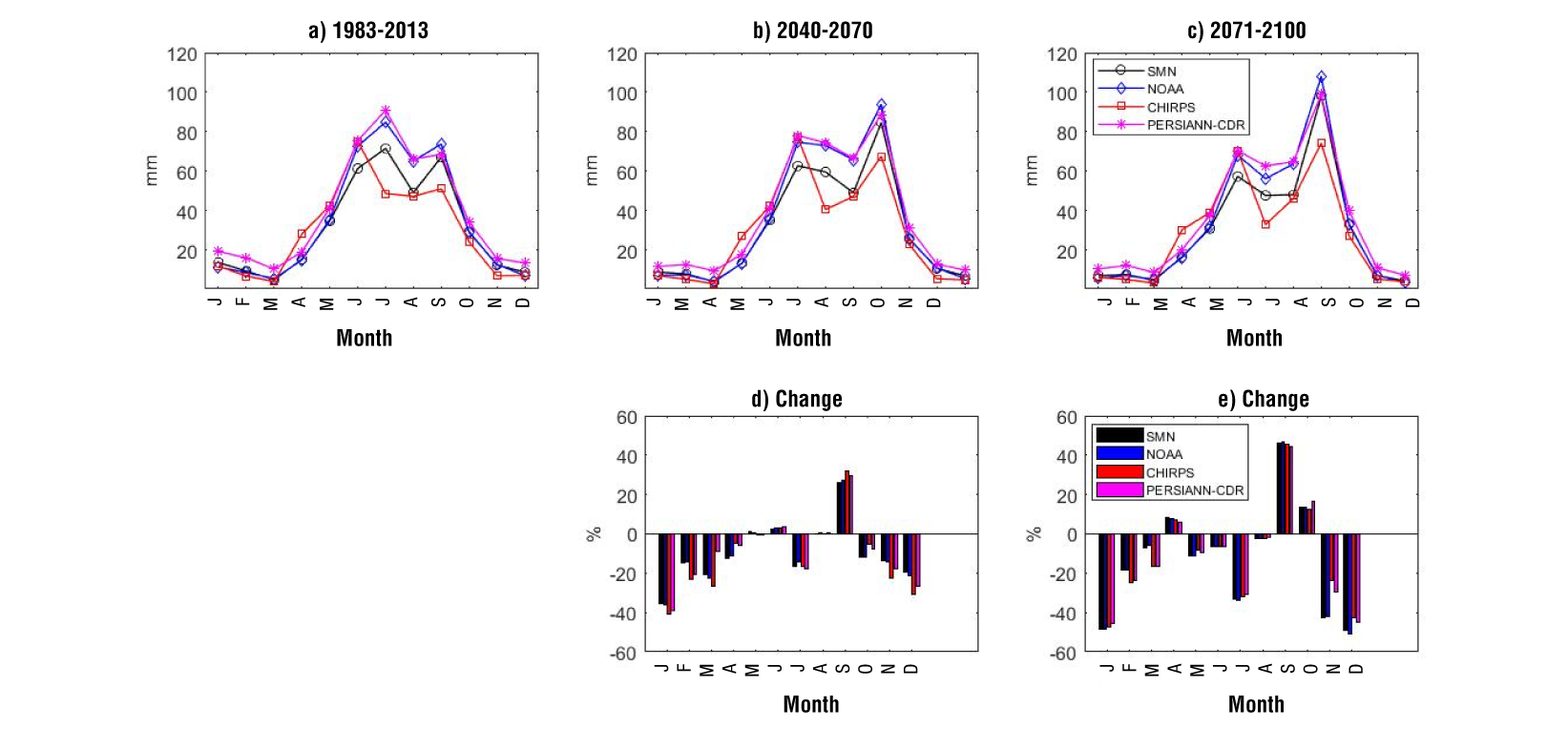
Figure 10 Annual cycles of precipitation for station 24069 in the historical period (a), the near future period 2040-2070 (b), and the far future period 2071-2100 (c), and the projected changes in precipitation between the historical and the future periods (d and e).
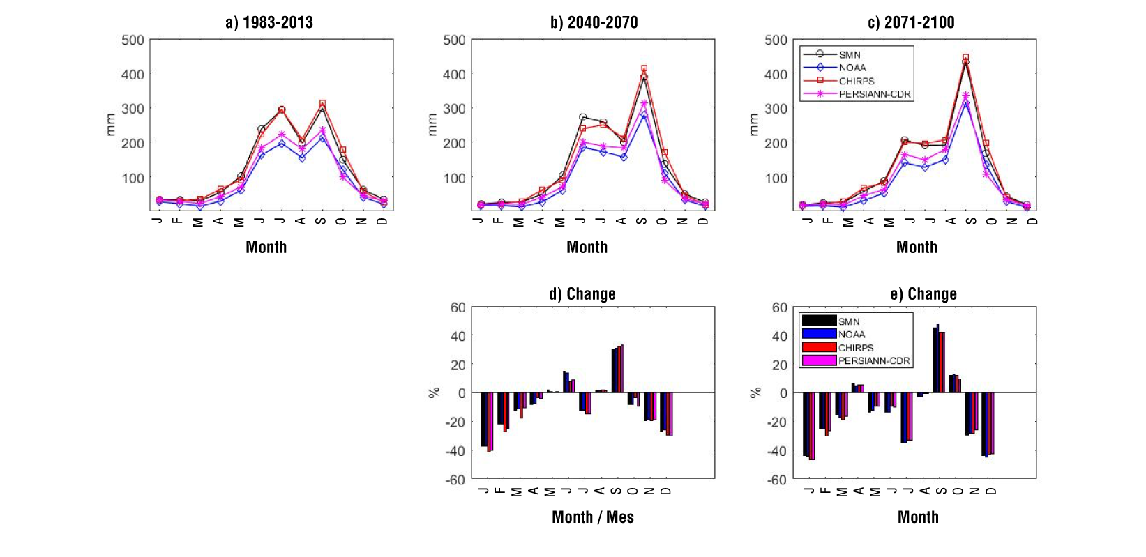
Figure 11 Annual cycles of precipitation for station 24005 in the historical period (a), the near future period 2040-2070 (b), and the far future period 2071-2100 (c), and the projected changes in precipitation between the historical and the future periods (d and e).
In future periods, the precipitation peaks are projected to change; for instance, the June peak decreases, and the September peak increases in both stations, especially in the far future period (Figures 10c and 11c). The change in precipitation (Figures10d and 11d) shows that, for most of the months, the simulations project a decrease, (especially in the dry months); for example, de change in January is about -38 and -47 % for the near and the far future respectively. The most important increase is projected in September, around 28 % in the near future, and around 46 % in the far future. The changes in precipitation among the datasets are very similar, despite the difference in annual cycles. Drought indicators were evaluated over the entire period 2040-2100 with the bias-corrected precipitation time series (Figure 12).
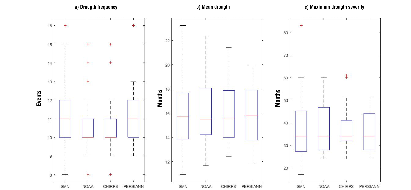
Figure 12 Drought indicators calculated for the period 2040-2100. Each boxplot is constructed with 35 results corresponding to the seven meteorological (or proxy) stations and the five climate simulations.
Drought indicators were evaluated for the entire 2040-2100 period with the bias corrected precipitations time-series and the results are presented in Figure 12. The median value in the indicators is similar among datasets; for example, the drought frequency is 10-11 events, the mean drought severity is approximately 16 months, and the maximum drought severity is about 35 months. The main difference is identified in the variability of the results, so NOAA data and CHIRPS data show a narrow boxplot in the indicators of drought frequency and maximum drought severity. On the other hand, climate simulations project that the arid climate type station 24069 would have the largest frequency of drought events, while the humid climate type station 24005 would experience the events with the highest drought severity.
Conclusions
Precipitation products should be evaluated in terms of the annual cycle representation and the amount and the variability of the precipitation. The results could differ between the climatic conditions of each study area.
The evaluation of the SPI obtained with precipitation products with the correlation coefficient is the most used in this type of study, but this statistic does not show the real performance of the forecast, therefore, the analysis with categorical scores is recommended.
Precipitation datasets show less variability than observations in historical period, which can affect the estimation of drought indicators when used to downscale and bias correct precipitation simulations in future period.
The NOAA Livneh dataset obtained the best results in terms of statistics and in reproducing the wet and dry periods, however, this database has the limitation of data availability (until 2013), and the spatial domain is restricted to North America. In contrast, the CHIRPS dataset is constantly updated, and the spatial domain is global.
Precipitation products can be used as an alternative when observed data are not available, but it is necessary to consider several products for monitoring droughts in the historical period, as well as in the estimation of droughts with future projections in order to evaluate the uncertainty.

