Original articles
Historical analysis of precipitation in Felipe Carrillo Puerto
Análisis histórico de la precipitación en Felipe Carrillo Puerto
Vargas Magaña, María Fernanda1
 http://orcid.org/0009-0005-8626-4377
Andrade-Velázquez, Mercedes2
http://orcid.org/0000-0001-9810-6003
http://orcid.org/0009-0005-8626-4377Andrade-Velázquez, Mercedes2
http://orcid.org/0000-0001-9810-6003
-
Publication dates-
January 20, 2025
Jan-Dec , 2024
- Article in PDF
- Article in XML
- Automatic translation
- Send this article by e-mail
- Share this article +
ABSTRACT
The present work deals with an analysis of the historical precipitation in the period 1972- 2012 of the stations FELIPE CARRILLO PUERTO (DGE) - QROO, X-PICHIL - QROO, and SEÑOR - QROO of the National Meteorological Service in the State of Quintana Roo to determine the dry and wet events of Felipe Carrillo Puerto town. Polygon areas surrounding the stations were defined using Voronoi diagrams and the standardized precipitation index (SPI) was calculated for the precipitation reported by each station. It was found that there are precipitation patterns changes between stations that may respond to the geographic factors of the area. It was proposed to calculate the SPI using an areal factor in the study area. The results show that the areal factor does not change the wet and dry events in the area, which allows us to have a distribution of precipitation in the area near the station. The precipitation patterns show for the study area greater dry events for the last years of the record, i.e. drought events in the area.
KEYWORDS::
Precipitation, SPI, Voronoi diagrams, Quintana Roo
Introduction
In the Mexican territory, various phenomena (hurricanes, severe storms, extreme droughts, fires, earthquakes, volcanoes) and geographical location are factors that influence the diversity of its climates and ecosystems (Gil et al., 2018). In Mexico, rainfall in most regions typically starts in May and usually continues until October, with September being the rainiest month nationwide. This is due to the influence of tropical systems like storms and hurricanes, the passage of cold fronts, and the arrival of the tropical convergence zone (ZTIC) (López Quiroz & Loranca Domínguez, 2022; Andrade-Velázquez, 2017).
-
Gil et al., 2018La vulnerabilidad de México ante el cambio climático: una revisión del Sistema Nacional de Protección Civil., 2018
-
López Quiroz & Loranca
Domínguez, 2022Reporte del clima en México, 2022
-
Andrade-Velázquez,
2017La cuenca del río Usumacinta desde la perspectiva del cambio climático. Instituto Mexicano de Tecnología del Agua, 2017
However, it is not uniform across the country, as precipitation records in Mexico indicate that the northern regions receive less rainfall than the southern areas. Another source of precipitation in the country is tropical cyclones. In the Pacific Ocean, this season begins on May 15th, while in the Atlantic Ocean, it begins on June 1st, and both coastlines conclude this season on November 30th (García, 1974).
-
García, 1974Distribución de la precipitación en la República MexicanaInvestigaciones Geográficas, Boletín del Instituto de Geografía, 1974
The southeast of Mexico is characterized by a tropical climate, primarily falling into the warm and humid category (INEGI, 2023). It is one of the areas of economic interest for the federal government, where the Tren Maya project is being developed (2023), aiming to boost the economy of local communities. Nevertheless, this region has been a national and international tourist attraction, with the beaches of Quintana Roo state being particularly popular (PROFECO, 2023). Villegas & Carrascal (1999) reported that tourist activities have had an environmental impact, leading to air and water pollution, alterations in vegetation cover, and changes in precipitation and daytime temperatures.
-
INEGI,
2023Quintana Roo, 2023
-
Tren Maya project is being
developed (2023)Secretaria de Turismo y Fonatur, 2023
-
PROFECO, 2023México Arena, sol y playas., 2023
-
Villegas & Carrascal (1999)Tourism development in Cancún, Quintana Roo and its consequences on vegetation.Investigaciones Geográficas, 1999
Quintana Roo is locatedin the eastern part of the Yucatan Peninsula, with a relatively homogeneous geological composition, mainly consisting of limestone strata. Its highest points approach around 300 meters above sea level (INEGI, 2002). Fragoso-Servón et al. (2014) report the existence of regional altitudinal zones with varying geodiversity, which is closely related to high biodiversity.
-
INEGI, 2002Estudio hidrológico del estado de Quintana Roo (I), 2002
-
Fragoso-Servón et al. (2014) Relación entre la geodiversidad de Quintana Roo y su biodiversidad. QuiveraRevista de Estudios Territoriales, 2014
The state of Quintana Roo experiences milder temperatures in January, while May, June, July, and August are the warmest months. It receives abundant precipitation, with the rainy season extending from May to October, and annual rainfall ranging from 800 to 1500 mm. The coastal areas of the state receive the highest amount of precipitation (INEGI, 2002). Precipitation patterns in the state follow the same regime as the southeast region, influenced by tropical cyclones and the intertropical convergence zone, occurring from May to November (Andrade-Velázquez & Montero-Martínez, 2023). Precipitation plays a crucial role in nourishing the inland water bodies. In Mexico, there are 653 water bodies, with 4 of them located on the Yucatan Peninsula (INEGI, 2018). Approximately 4,000,000 people depend on these water bodies, making water availability in this area one of the most critical in all of Mexico (CONAGUA, 2018). In Quintana Roo, the aquifer serves as the primary source of water supply for communities and urban areas (Sánchez, et al. 2016).
-
INEGI, 2002Estudio hidrológico del estado de Quintana Roo (I), 2002
-
Andrade-Velázquez & Montero-Martínez,
2023Historical and projected trends of the mean surface temperature in South-Southeast Mexico using ERA5 and CMIP6.Climate, 2023
-
INEGI, 2018Agua. Cuéntame de México., 2018
-
CONAGUA, 2018Estadísticas del agua en México, 2018
-
Sánchez, et al. 2016Calidad del agua subterránea: acuífero sur de Quintana Roo, México.Tecnología y Ciencias del Agua, 2016
The predominant culture in the area is Maya, and several municipalities of local interest due to their cultural richness can be found among its communities, with the municipality of Felipe Carrillo Puerto being one of them (Felipe Carrillo Puerto, 2023).
-
Felipe Carrillo Puerto, 2023Ayuntamiento de Felipe Carrillo Puerto, 2023
This study is focused on determining wet and dry events in the municipality of Felipe Carrillo Puerto. To achieve this, the Standardized Precipitation Index (SPI) and the proposed areal factor are utilized. The methodology is described in the following section, followed by the presentation of results, and, finally, the conclusions.
Material and Methods
Study zone
Felipe Carrillo Puerto is located in the state of Quintana Roo, Mexico; in the central region of the state, with geographic coordinates: latitude: 19.578611°N, longitude: 88.045278°W, and an altitude between 0 and 100 meters. It belongs to the Hydrological Region of Eastern Yucatan (Quintana Roo) and the Bay of Chetumal. It has some bodies of surface water, although its soil is formed by the same limestone rock as the rest of the Yucatan Peninsula, which prevents surface water flows (INEGI, 2009).
-
INEGI, 2009Compendio de información geográfica municipal. Felipe Carrillo Puerto, Quintana Roo., 2009
Data
Monthly time series data of precipitation were used; this data was collected from the CLICOM network of surface weather stations located in Felipe Carrillo Puerto, Quintana Roo (Figure 1).
-
CLICOM, 00000000
Thumbnail
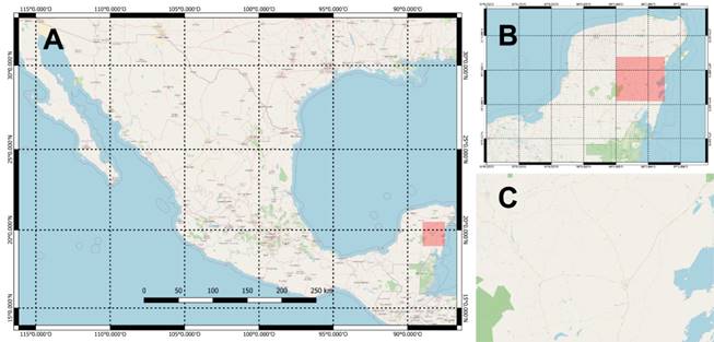
Figure 1
Location of the study area (A) Mexican territory (B) Yucatan Peninsula. (C) Felipe Carrillo Puerto, Quintana Roo.
Location of the study area (A) Mexican territory (B) Yucatan Peninsula. (C) Felipe Carrillo Puerto, Quintana Roo.
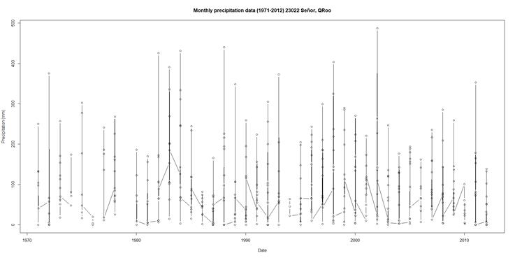
In the Table 1 displays the distribution of complete data obtained from each station and in the figures (Figure 2, Figure 3, Figure 4) we observe the graphs of monthly precipitation for each station using the complete data. Similarly, you can observe a percentage of data in the table, this is due to the fact that the blank spaces in the graphs are missing data.
It is worth mentioning that the stations have variations in the data year ranges, so it was decided to truncate the ranges and use data from the same year (1972 - 2012).
| NUMBER | STATION NAME | RANGE OF YEARS OF DATA | PORCENTAGE OF DATA (%) | AMOUNT OF DATA CONTAINED FROM 1972 TO 2012 |
|---|---|---|---|---|
| 23003 | FELIPE CARRILLO PUERTO (DGE) - QROO | 1952 - 2012 | 97.24 | 472 |
| 23031 | X-PICHIL - QROO | 1971 - 2012 | 85.37 | 486 |
| 23022 | SEÑOR - QROO | 1961 - 2012 | 99.04 | 419 |
Thumbnail
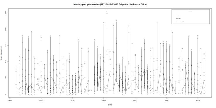
Figure 2
Monthly precipitation of the station FELIPE CARRILLO PUERTO (DGE) - QROO from 1952 to 2012.
Monthly precipitation of the station FELIPE CARRILLO PUERTO (DGE) - QROO from 1952 to 2012.
Thumbnail
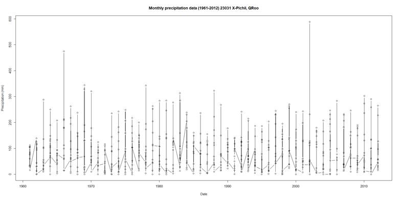
Figure 3
Monthly precipitation of the X-PICHIL - QROO station from 1971 to 2012.
Monthly precipitation of the X-PICHIL - QROO station from 1971 to 2012.
Thumbnail
Voronoi diagram
To determine the mean precipitation over the study area, the Voronoi over the study area was determined using the Voronoi Diagram method. The Voronoi Diagram was defined in 1907 by a Ukrainian mathematician by the name of Geogy Vornoi. Although it is also known as Thiessen Polygons after the American meteorologist Alfred Thiessen. American meteorologist Alfred Thiessen, who applied this method for weather prediction in weather prediction in 1911 (Fortune, 1986).
-
Fortune, 1986A sweepline algorithm for Voronoi diagrams., 1986
A Voronoi Diagram is a type of pattern that is created when covering a surface considering distance. It results in a geometric formation that allows for the partitioning of the plane. This partition is based on dividing the geometric plane into as many regions as there are points, such that each point is designated the region consisting of everything closer to it than to any other point (De Berg et al., 2008).
-
De Berg et al., 2008Computational Geometry: Algorithms and Applications., 2008
This method is used when the study area has an irregular distribution of weather stations. It is based on examining the precipitation value of each climatological station in relation to its area of influence (Moreno Rodríguez & Montero Torres, 2016).
-
Moreno Rodríguez & Montero Torres,
2016Evaluación de v aluación de variables climáticas par ariables climáticas para cuantificar el r a cuantificar el recurso hídrico disponible en la cuenca media del Río Ranchería, 2016
Mean precipitation
The average precipitation is obtained by calculating the average of the three stations. We propose that the calculation be as follows.
The average precipitation will result from the sum of the product of the precipitation of each station by the quotient of the area of each station by the area in general:
Where:
A i : Polygon area corresponding to the station i.
A: Total area of the study zone.
n: Number of stations.
Standardized precipitation index
The Standardized Precipitation Index (SPI), developed in 1993 by McKee and colleagues, aims to enhance the detection of drought onset and monitoring. It is primarily employed to assess the occurrence of significant precipitation deficits or excesses within a specific region across various time scales (McKee et al., 1993). SPI calculations span time scales ranging from 3 to 48 months. SPI values range from +3 to -3; a drought period is considered when consecutive SPI values are negative, and the drought period concludes when the SPI becomes positive (NCAR, 2017).
-
McKee et al., 1993The relationship of drought frequency and duration to time scales, 1993
-
NCAR, 2017Standardized Precipitation Index (SPI). Climate Data Guide., 2017
The following table 2 indicates the range of the Standardized Precipitation Index as used by McKee and others (McKee et al., 1993):
-
McKee et al., 1993The relationship of drought frequency and duration to time scales, 1993
Table 2
Range of the Standardized Precipitation Index.
Range of the Standardized Precipitation Index.
| VALUE | CATEGORY |
|---|---|
| > 2.0 | Extreme humidity |
| 2.0 to 1.5 | Severe humidity |
| 1.5 to 1.0 | Moderate humidity |
| 1.0 to -1.0 | Near normal |
| -1.0 to -1.5 | Moderate drought |
| -1.5 to -2.0 | Severe drought |
| < -2.0 | Extreme drought |
-
McKee et al.
(1993)The relationship of drought frequency and duration to time scales, 1993
On a relatively short time scale (1, 3, or 6 months), precipitation anomalies can occur that may alter soil moisture conditions. Conversely, on a time scale of 12, 24, 36, or 48 months, rainfall anomalies are revealed due to changes in surface and subsurface currents, as well as reservoirs (Svoboda & Hayes, 2012).
-
Svoboda & Hayes, 2012Índice normalizado de precipitación, Guía del usuario, 2012
The calculation of the Standardized Precipitation Index is based on the monthly precipitation record, where each month establishes a new value based on the previous months. Each of these data points is adjusted to the "Gamma" function, aiming to define the relationship between probability and precipitation (McKee et al., 1993).
-
McKee et al., 1993The relationship of drought frequency and duration to time scales, 1993
The Gamma distribution is defined by its frequency or probability density
function (for details, refer to Annex A):
Where
In this case, the parameters
Results
In Figure 5 we observe the geographic distribution and the area of interest of the three stations, determined by the Voronoi diagram. In the following Table 4, the area of each polygon, its percentage of the total area, and the corresponding areal average are shown. The total area of the Voronoi diagram is 2568.88 km².
Thumbnail
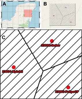
Figure 5
Voronoi diagram: (A) location in Mexico, (B) location at study zone, and (C) the amplified Voronoi diagram.
Voronoi diagram: (A) location in Mexico, (B) location at study zone, and (C) the amplified Voronoi diagram.
In Figure 6, the time series of monthly precipitation for each station is presented. The maximum recorded precipitation value from 1972 to 2012 in Figure 6-A is 506.9 mm, in Figure 6-B is 588.5 mm, and in Figure 6-C is 487.7 mm. It is worth mentioning that the maximum values in Figure 6-A and 6-B were recorded in the same month and year (September 2002). On the other hand, in the following Table 4, we have the overall average precipitation for each station, with the station closest to the point of interest (FELIPE CARRILLO PUERTO (DGE) - QROO) having the highest overall average precipitation. However, according to the Voronoi diagram created, this same station has the polygon with the smallest area.
We observe that the area distribution is greater for the X-PICHIL - QROO station, accounting for 40% of the total, while the area of the station closest to the study area is just over 26%. This will determine the precipitation distribution in the area based on its percentage.
In Table 3, we see that the average precipitation for Felipe Carrillo Puerto is 30 mm per square kilometer. This result will be discussed further.
Table 3
Data for each station.
Data for each station.
| 23003-FELIPE CARRILLO PUERTO (DGE) - QROO | 23031-X-PICHIL - QROO | 23022-SEÑOR - QROO | |
| Area (km2) | 684.52 | 1054.45 | 829.91 |
| Areal percentage | 26.65% | 41.05% | 32.30% |
| Areal average precipitation (mm/km2) | 30.044 | 37.328 | 31.428 |
Thumbnail
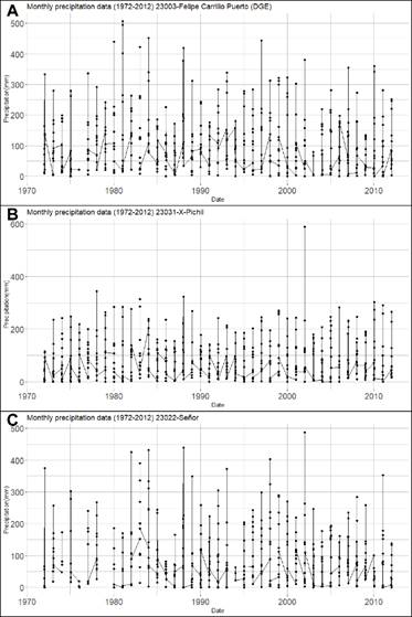
Figure 6
Monthly precipitation time series from 1972 to 2012 for each station studied (A) Station FELIPE CARRILLO PUERTO (DGE) - QROO. (B) Station X-PICHIL - QROO. (C) Station SEÑOR - QROO.
Monthly precipitation time series from 1972 to 2012 for each station studied (A) Station FELIPE CARRILLO PUERTO (DGE) - QROO. (B) Station X-PICHIL - QROO. (C) Station SEÑOR - QROO.
Figures 6A and 6C exhibit similar patterns, with the rainiest period occurring between 1980 and 1985. However, in Figure 6B, precipitation remains nearly constant, meaning it does not vary over the years. It is important to note that in this graph, there are many empty months between 1972 and 1980, indicating that precipitation was not recorded during these months for unknown reasons.
From the same figures, we observe that, except for the maximum events, all three stations show similar precipitation trends.
Figure 7 displays the result of the average monthly precipitation among the three studied stations (Station 23003-FELIPE CARRILLO PUERTO (DGE), Station 23031-X-PICHIL - QROO, Station 23022-SEÑOR - QROO), with the maximum precipitation value reaching 485.5 mm in September 2002. Table 5 reports the monthly precipitation averages over the 40-year period (1972-2012). In the same table, we observe that the highest precipitation occurs at the FELIPE CARRILLO PUERTO station (DGE23003-Felipe Carrillo Puerto (DGE).
Table 5 shows the average precipitation for each month from 1972 to 2012 for each station. This table allows us to observe the increase or decrease in precipitation in all months of the year.
The average monthly precipitation for each station follows the same pattern for all three stations. This indicates that the precipitation climatology is consistent in the surrounding region of the study area. Precipitation occurs throughout the year, with maximums of around 40 mm in winter months, while in summer, precipitation is higher from May to October, exceeding 100 mm, as the Atlantic hurricane season occurs from June to November (CONAGUA, 2023).
-
CONAGUA,
2023Temporada Ciclones Tropicales 2023, 2023
Thumbnail
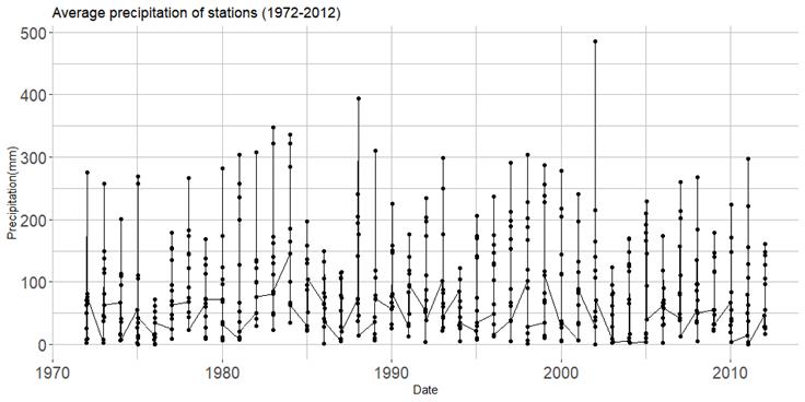
Figure 7
Time series of average precipitation for the three stations studied from 1972 to 2012.
Time series of average precipitation for the three stations studied from 1972 to 2012.
Table 4
General mean precipitation in each meteorological station from 1972 to 2012.
General mean precipitation in each meteorological station from 1972 to 2012.
| 23003-FELIPE CARRILLO PUERTO (DGE) - QROO | 23031-X-PICHIL - QROO | 23022-SEÑOR - QROO |
|---|---|---|
| 112.75 | 90.94 | 97.28 |
Table 5
Mean precipitation in each month of each of the stations from 1972 to 2012.
Mean precipitation in each month of each of the stations from 1972 to 2012.
| Mean precipitation (mm) in each month of 23003-FELIPE CARRILLO PUERTO (DGE) - QROO from 1972 to 201 | |||||||||||
|---|---|---|---|---|---|---|---|---|---|---|---|
| jan | feb | mar | apr | may | jun | jul | aug | sep | oct | nov | dec |
| 54.82 | 49.77 | 39.36 | 40.53 | 116.51 | 173.88 | 149.11 | 159.88 | 206.17 | 173.78 | 82.79 | 55.67 |
| Mean precipitation (mm) in each month of 23031-X-PICHIL - QROO from 1972 to 2012 | |||||||||||
| 47.07 | 37.34 | 31.97 | 36.92 | 93.19 | 136.99 | 132.55 | 142.74 | 192.16 | 130.36 | 69.58 | 43.22 |
| Mean precipitation (mm) in each month of 23022-SEÑOR - QROO from 1972 to 2012 | |||||||||||
| 43.77 | 40.85 | 32.14 | 46.33 | 105.81 | 151.74 | 113.83 | 136.66 | 216.93 | 150.03 | 79.14 | 47.4 |
Below are the results of the Standardized Precipitation Index (SPI) calculations for each station. Analyzing each of these figures, it is observed that there are different patterns in dry and wet events for each station. The SPI was calculated for a 3-month, 12-month, and 36-month window for a short and long-term analysis of dry and wet events.
The station closest to the point of interest, 23003-FELIPE CARRILLO PUERTO (DGE) - QROO (Figure 8), has values indicating extreme drought (SPI less than -2.0), and these periods are very short, ranging from one to two years. However, wet periods span 2 to 3 years, with values indicating extreme moisture (SPI greater than 2.0). This is particularly evident in the calculation of SPI-12 (12 months).
In contrast, with the same SPI-12, at station 23031-X-PICHIL - QROO (Figure 9), the intensity of droughts does not vary much. Throughout the period from 1972 to 2012, it maintains SPI values mostly between Near Normal (SPI from 1.0 to -1.0) and Mild Drought (SPI from -1.0 to -1.5).
The station SEÑOR - QROO23022 shows, for SPI-12 (Figure 10), that the intensity of droughts remains similar to the previous station. This station has the least amount of recorded data.
It is worth mentioning that the Standardized Precipitation Index (SPI) with periods of 36 months (Figure 10), could not be determined for the first 10 years, due to the fact that there is a lot of missing data in that period of time.
Thumbnail
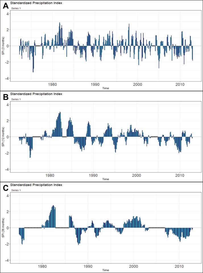
Figure 8
Standardized precipitation index (SPI) of (A) 3 months, (B) 12 months and (C) 36 months of the station FELIPE CARRILLO PUERTO (DGE) - QROO from 1972 to 2012.
Standardized precipitation index (SPI) of (A) 3 months, (B) 12 months and (C) 36 months of the station FELIPE CARRILLO PUERTO (DGE) - QROO from 1972 to 2012.
Thumbnail
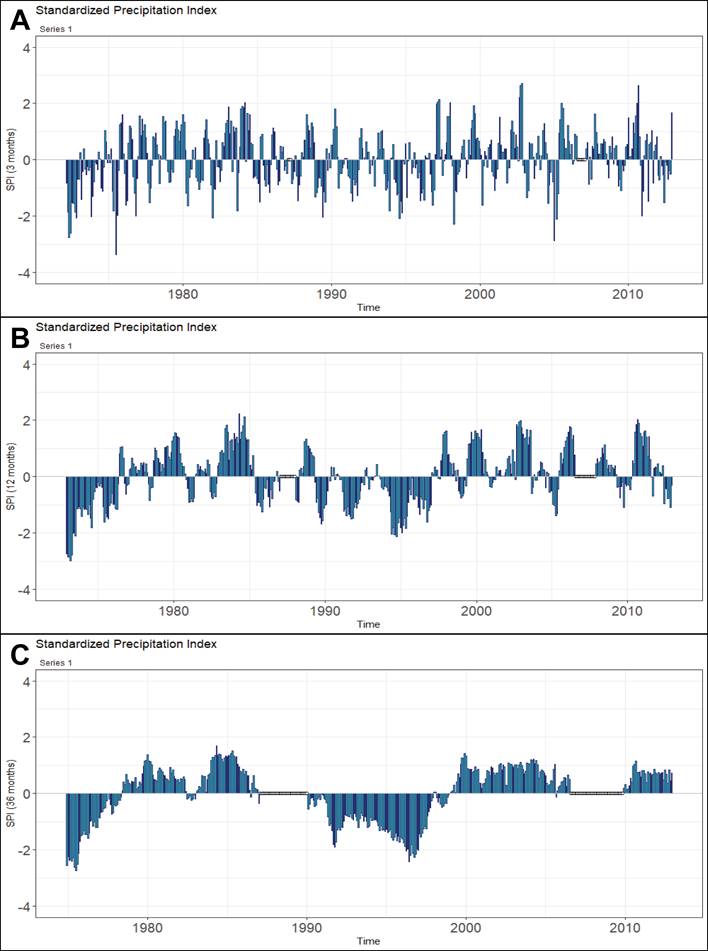
Figure 9
Standardized precipitation index (SPI) for (A) 3 months, (B) 12 months and (C) 36 months for the X-PICHIL - QROO station from 1972 to 2012.
Standardized precipitation index (SPI) for (A) 3 months, (B) 12 months and (C) 36 months for the X-PICHIL - QROO station from 1972 to 2012.
Thumbnail
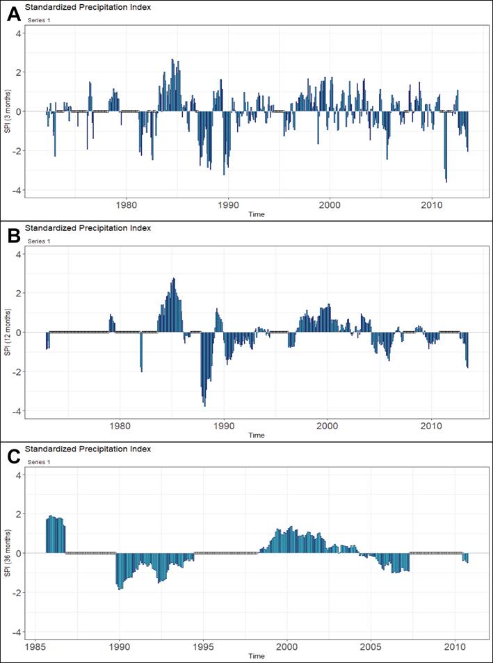
Figure 10
Standardized precipitation index (SPI) for (A) 3 months, (B) 12 months and (C) 36 months for the SEÑOR - QROO station from 1972 to 2012.
Standardized precipitation index (SPI) for (A) 3 months, (B) 12 months and (C) 36 months for the SEÑOR - QROO station from 1972 to 2012.
The following figures (Figure 11, Figure 12, and Figure 13) represent the results of the Standardized Precipitation Index (SPI) for the average precipitation of the three studied stations, the average precipitation with the areal factor of the study area, and the areal precipitation in the zone of the station nearest to the point of interest.
These SPI values were calculated for periods of 3 months (Figure 11), 12 months (Figure 12), and 36 months (Figure 13). Analyzing these three calculations, it is observed that the correction of the areal factor preserves the patterns of the events; only the intensity changes, as the areal factor distributes precipitation in the area assigned by each Voronoi diagram.
Thumbnail
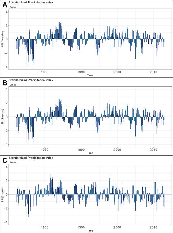
Figure 11
Standardized precipitation index (SPI) for 3 months of the (A) average precipitation, (B) areal average precipitation and (C) areal precipitation of the FELIPE CARRILLO PUERTO (DGE) - QROO station from 1972 to 2012.
Standardized precipitation index (SPI) for 3 months of the (A) average precipitation, (B) areal average precipitation and (C) areal precipitation of the FELIPE CARRILLO PUERTO (DGE) - QROO station from 1972 to 2012.
Thumbnail
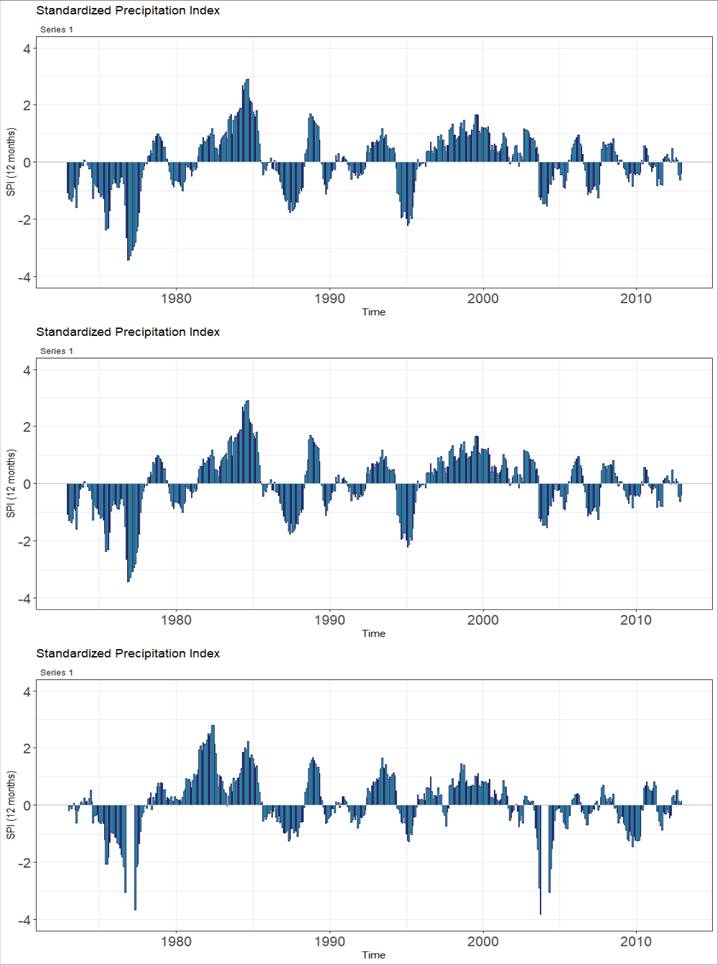
Figure 12
12-month Standardized Precipitation Index (SPI) of the (A) average precipitation, (B) areal average precipitation and (C) areal precipitation of the FELIPE CARRILLO PUERTO (DGE) - QRoo station from 1972 to 2012.
12-month Standardized Precipitation Index (SPI) of the (A) average precipitation, (B) areal average precipitation and (C) areal precipitation of the FELIPE CARRILLO PUERTO (DGE) - QRoo station from 1972 to 2012.
Thumbnail
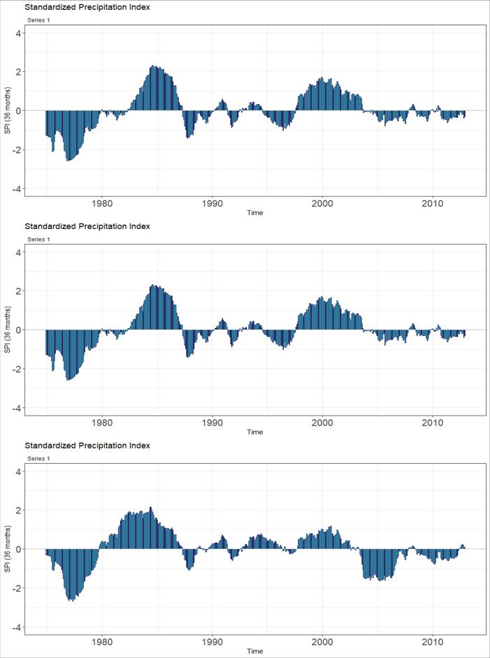
Figure 13
Standardized precipitation index (SPI) of 36 months of the (A) average precipitation, (B) areal average precipitation and (C) areal precipitation of the station FELIPE CARRILLO PUERTO (DGE) - QROO from 1972 to 2012.
Standardized precipitation index (SPI) of 36 months of the (A) average precipitation, (B) areal average precipitation and (C) areal precipitation of the station FELIPE CARRILLO PUERTO (DGE) - QROO from 1972 to 2012.
Discussion
The present study has conducted a historical analysis of precipitation in the town of Felipe Carrillo Puerto using information from three stations surrounding the study area and proposing the areal factor (Ai/AT) for the distribution of precipitation in that zone. This proposal allows us to obtain the average precipitation in Felipe Carrillo Puerto and identify its precipitation patterns over the 40-year period from 1972 to 2012, as recommended by the World Meteorological Organization (OMM, 1994).
-
OMM, 1994Guía de prácticas Hidrológicas: adquisición y proceso de datos, análisis, predicción y otras aplicaciones., 1994
The behavior of precipitation throughout the annual cycle over these 40 years was determined, revealing an average precipitation of 40 mm for winter months and over 100 mm in summer months. This corresponds to the hydrometeorological events in southeastern Mexico, such as the passage of cold fronts in winter and the presence of tropical cyclones, combined with the intertropical convergence zone in summer (Andrade-Velázquez, 2017).
-
Andrade-Velázquez, 2017La cuenca del río Usumacinta desde la perspectiva del cambio climático. Instituto Mexicano de Tecnología del Agua, 2017
On the other hand, using the Standardized Precipitation Index (SPI) calculations for temporal windows of 3 months, 12 months, and 36 months, dry and wet events in the study area were identified. With SPI-3, it was found that seasonal events were more intense in the 1980s, while in recent years (2010s), they have been less intense, both in terms of moisture and dryness. SPI-12 provided similar information on an annual basis, extending its duration to a year, allowing the identification of dry and wet years. Meanwhile, SPI-36 provided the duration of long episodes lasting 3 years for dry and wet events. In this case, for the station near Felipe Carrillo Puerto, predominantly dry events have occurred in recent years, contrary to what is reported by the X-PICHIL station, where wet events are observed.
In Figure 14, we observe that while Felipe Carrillo Puerto is closer to the coast, X-PICHIL is farther inland. We attribute this contrast between events to local factors, possibly the type of vegetation and topography in each region. In the case of the station SEÑOR, it is located to the north of the town of Felipe Carrillo Puerto. Additionally, the lack of information in its records for some months during the 1972-2012 period prevents us from having a reference for SPI-12 as SPI-36.
Thumbnail
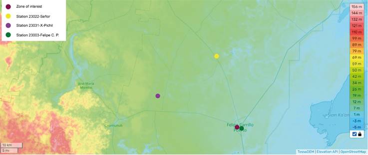
Figure 14
Topographic map of altitude and relief of Quintana Roo.
Topographic map of altitude and relief of Quintana Roo.
Therefore, it is advisable to have a precipitation analysis with an areal factor for the study area in relation to the nearest station rather than obtaining simple average precipitation. Figures 119-131 show the SPI-3, SPI-12, and SPI-36 calculations, respectively, for the simple average of the three stations (Section A), for the areal average of the three stations (Section B), and for only the Felipe Carrillo Puerto station (Section C). We notice that while graphs A and B maintain the patterns of dry and wet events, only the intensity is modified by the factor (1/AT). In the case of graph C, we observe changes in the timing of dry and wet events, but this is due to considering only one of the stations. This provides greater reliability in the analysis since it is the closest station, meaning we have the same information only modified by a factor of (Ai/AT). This result allows us to ensure that precipitation at any point within the polygon of the Felipe Carrillo Puerto station will exhibit behavior close to this station, whose local conditions are similar, as opposed to obtaining behavior from the average of the three stations, where all three stations show different precipitation patterns. This demonstrates that weighted precipitation analysis with an areal factor enables the determination of dry and wet events in the study area according to the proposed methodology.
On the other hand, this analysis shows that dry and wet events in the study area are more intense, ranging from severe to extreme, according to McKee et al. (1993), before 1985. Subsequently, these events range from normal to severe. It should be noted that Magaña et al. (2003) has indicated that the El Niño-Southern Oscillation (ENSO) influences the occurrence of dry and wet events in Mexico. Méndez and Magaña (2010) report the influence of the combination of ENSO, the Pacific Decadal Oscillation (PDO), and the Atlantic Multidecadal Oscillation (AMO) in a geographical dipole (North-South) in the country. Other authors report similar studies in other parts of the world (Abiy et al. 2019; Jia et al., 2021). Figure 15 shows the behavior of the Oceanic Niño Index (ONI; NOAA, 2023), indicating El Niño (>0.5°C) and La Niña (<0.5°C) episodes. We observe that the variability of SPI-12 follows the behavior of the index, leading us to assume an influence of ENSO in the study area. While Olivera-Villaroel et al. (2021) report that before 1985, the PDO was in a positive phase and later in a negative phase. Taking into account the aforementioned studies, we suggest that PDO influences the intensity of dry and wet events in precipitation in the study area. These results are indicated for the first time in the study area in the state of Quintana Roo. It should be noted that there are studies at the national level (Magaña et al. 2003; Bravo-Cabrera et al. 2017), in the northern region (Hallack-Alegria & Watkinz, 2007; Méndez et al. 2010), or the southeast in the Grijalva-Usumacinta Basin (Golicher et al., 2006; Andrade-Velazquez & Medrano-Pérez, 2020). However, for the study area, this work provides a climatic analysis of precipitation.
-
McKee et al. (1993)The relationship of drought frequency and duration to time scales, 1993
-
Magaña et al. (2003)Impact of El Niño on precipitation in MexicoGeofísica Internacional, 2003
-
Méndez and Magaña (2010)Regional aspects of prolonged meteorological droughts over Mexico and Central AmericaJournal of Climate, 2010
-
Abiy et al. 2019Teleconnection of regional drought to ENSO, PDO, and AMO: Southern Florida and the EvergladesAtmosphere, 2019
-
Jia et al., 2021Drought variability and its connection with large-scale atmospheric circulations in Haihe River BasinWater Science and Engineering, 2021
-
NOAA, 2023Cold & Warm Episodes by Season., 2023
-
Olivera-Villaroel et al. (2021)Exposición a cambios en el clima en BoliviaTecnología Y Ciencias Del Agua, 2021
-
Magaña et al. 2003Impact of El Niño on precipitation in MexicoGeofísica Internacional, 2003
-
Bravo-Cabrera et al. 2017Effects of El Niño in Mexico during rainy and dry seasons: an extended treatmentAtmosfera, 2017
-
Hallack-Alegria & Watkinz, 2007Annual and Warm Season Drought Intensity-Duration-Frequency Analysis for Sonora, MexicoJournal of Climate, 2007
-
Méndez et al. 2010Teleconnection of the Pacific Decadal Oscillation (PDO) to the precipitation and temperature in MexicoInvestigaciones geográficas, 2010
-
Golicher et al.,
2006Correlations between precipitation patterns in southern mexico and the el niño sea surface temperature indexInterciencia, 2006
-
Andrade-Velazquez &
Medrano-Pérez, 2020Patrones de precipitación en las cuencas Usumacinta y Grijalva (sur de México) bajo un clima cambiante.Revista Bio Ciencias, 2020
Thumbnail
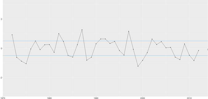
Figure 15
Oceanic El Niño index plot. Source: NOAA, 2023.
Oceanic El Niño index plot. Source: NOAA, 2023.
Conclusions
In conclusion, a study similar to the one presented here has not been conducted for the study area, allowing us to characterize precipitation to understand the recent climate in the town of Felipe Carrillo Puerto. The analysis demonstrated that averaging data from the three stations helps smooth out patterns, making it preferable to use an areal factor by assigning an area to the nearest station to determine precipitation at points within that area. Lastly, the study suggests the influence of ENSO and PDO on precipitation in the study area.
We observe that, in the town of Felipe Carrillo Puerto, drier events have occurred more frequently than wetter ones in recent years from 2007 to 2012. This information contributes to understanding the local climate and its potential effects on the town. We believe this may explain the drying of bodies of water, such as the case of the "La Cruz Parlante" cenote. However, this study solely focuses on climatic analysis to provide information for application or impact studies. It requires complementation with social and environmental studies, which is beyond the scope of the authors.
Acknowledgments
We appreciate the internship program between the Division of Basic Sciences at the Universidad Juárez Autónoma de Tabasco and the Center for Global Change and Sustainability. Thanks to the Researchers for Mexico program from the National Council for Humanities, Sciences, and Technologies. To Dr. Martín José Montero-Martínez for some comments and suggestions.
References
- Abiy, A. Z., Melesse, A. M., & Abtew, W. (2019). Teleconnection of regional drought to ENSO, PDO, and AMO: Southern Florida and the Everglades. Atmosphere, 10(6), 295. https://doi.org/10.3390/atmos10060295 Links
- Andrade-Velázquez, M., & Montero-Martínez, M. J. (2023). Historical and projected trends of the mean surface temperature in South-Southeast Mexico using ERA5 and CMIP6. Climate, 11(5), 111. https://doi.org/10.3390/cli11050111 Links
- Andrade-Velázquez, M., & Pérez, O. R. M. (2020). Patrones de precipitación en las cuencas Usumacinta y Grijalva (sur de México) bajo un clima cambiante. Revista Bio Ciencias, 7(1). https://doi.org/10.15741/revbio.07.e905 Links
- Andrade-Velázquez, M., Soares, D., & García García, A. (2017). La cuenca del río Usumacinta desde la perspectiva del cambio climático. Instituto Mexicano de Tecnología del Agua. https://www.imta.gob.mx/biblioteca/libros_html/la-cuenca-rio-usumacinta/files/assets/basic-html/page58.html ISBN 978-607-9368-81-4 Links
- Base de Datos del CLICOM. (s. f.). CICESE. http://clicom-mex.cicese.mx/mapa.html Links
- Bravo-Cabrera, J. L., Azpra-Romero, E., Zarraluqui-Such, V., & Gay-García, C. (2017). Effects of El Niño in Mexico during rainy and dry seasons: an extended treatment. Atmosfera, 30(3). https://doi.org/10.20937/atm.2017.30.03.03 Links
- Comisión Nacional del Agua [CONAGUA]. (2018). Estadísticas del agua en México. https://sina.conagua.gob.mx/publicaciones/EAM_2019.pdf Links
- Comisión Nacional del Agua [CONAGUA]. (2023). Temporada Ciclones Tropicales 2023. https://smn.conagua.gob.mx/es/ciclones-tropicales/temporada-ciclones-tropicales-2023 Links
- De Berg, M., Cheong, O., Van Kreveld, M., & Overmars, M. (2008). Computational Geometry: Algorithms and Applications. Springer Science & Business Media. ISBN 3-540-65620-0 Links
- Edwards, D. C., & McKee T.B (1997). Characteristics of 20th century drought in the United States at multiple time scales. Atmospheric Science Paper, 634, 1-30 http://hdl.handle.net/10217/170176 Links
- Felipe Carrillo Puerto. (2023). Ayuntamiento de Felipe Carrillo Puerto. https://www.felipecarrillopuerto.gob.mx/ Links
- Fortune, S. (1986). A sweepline algorithm for Voronoi diagrams. Proceedings of the second annual symposium on Computational geometry - SCG ’86. https://doi.org/10.1145/10515.10549 Links
- Fragoso-Servón, P., Pereira, A., Frausto, O., & Bautista, F. (2014). Relación entre la geodiversidad de Quintana Roo y su biodiversidad. Quivera. Revista de Estudios Territoriales, 16 (1), 97-125. https://www.redalyc.org/pdf/401/40132130006.pdf Links
- García, E. (1974). Distribución de la precipitación en la República Mexicana. Investigaciones Geográficas, Boletín del Instituto de Geografía, 50. https://doi.org/10.14350/rig.30432 Links
- Gil, R. Z., Pineda, A. H., Correa, M. K. S., & Ramírez, M. C. S. (2018). La vulnerabilidad de México ante el cambio climático: una revisión del Sistema Nacional de Protección Civil. Instituto Belisario Domínguez, 1. http://bibliodigitalibd.senado.gob.mx/handle/123456789/4108 ISBN 978-607-8620-05-0 Links
- Golicher, J. D., Ramírez‐Marcial, N., & Levy-Tacher, S. I. (2006). Correlations between precipitation patterns in southern mexico and the el niño sea surface temperature index. Interciencia, 31(2), 80-86. http://www.interciencia.org/v31_02/080.pdf Links
- Hallack-Alegría, M., & Watkins, D. (2007). Annual and Warm Season Drought Intensity-Duration-Frequency Analysis for Sonora, Mexico. Journal of Climate , 20(9), 1897-1909. https://doi.org/10.1175/jcli4101.1 Links
- Instituto Nacional de Geografía y Estadística [INEGI]. (2018). Agua. Cuéntame de México. https://cuentame.inegi.org.mx/territorio/agua/cuerpos.aspx?tema=T Links
- Instituto Nacional de Geografía y Estadística [INEGI]. (2023). Quintana Roo. https://cuentame.inegi.org.mx/monografias/informacion/qroo/territorio/clima.aspx?tema=me Links
- Instituto Nacional de Geografía y Estadística [INEGI]. (2002). Estudio hidrológico del estado de Quintana Roo (I). ISBN 970-13-3737-9 https://www.inegi.org.mx/contenidos/productos/prod_serv/contenidos/espanol/bvinegi/productos/historicos/2104/702825224196/702825224196_1.pdf Links
- Instituto Nacional de Geografía y Estadística [INEGI]. (2009). Compendio de información geográfica municipal. Felipe Carrillo Puerto, Quintana Roo. https://www.inegi.org.mx/contenidos/app/mexicocifras/datos_geograficos/23/23002.pdf Links
- Jia, W., Wang, W., Huang, Y., Ding, Y., Fu, J., & Chen, Z. (2021). Drought variability and its connection with large-scale atmospheric circulations in Haihe River Basin. Water Science and Engineering, 14(1), 1-16. https://doi.org/10.1016/j.wse.2020.12.007 Links
- López Quiroz, M., & Loranca Domínguez, Y. (2022). Reporte del clima en México. CONAGUA, 8. https://smn.conagua.gob.mx/tools/DATA/Climatolog%C3%ADa/Diagn%C3%B3stico%20Atmosf%C3%A9rico/Reporte%20del%20Clima%20en%20M%C3%A9xico/RC-Agosto22.pdf Links
- Magaña, V., Vázquez, J., Pérez, J. L., & Pérez, J. (2003). Impact of El Niño on precipitation in Mexico. Geofísica Internacional, 42(3), 313-330. https://doi.org/10.22201/igeof.00167169p.2003.42.3.949 Links
- McKee, T. B., Doesken, N. J., & Kleist, J. (1993). The relationship of drought frequency and duration to time scales. Eighth Conference on Applied Climatology. http://clima1.cptec.inpe.br/~rclima1/pdf/paper_spi.pdf Links
- Méndez, J., Ramírez, A., Cornejo, E., Zárate, A., & Cavazos, T. (2010). Teleconnection of the Pacific Decadal Oscillation (PDO) to the precipitation and temperature in Mexico. Investigaciones geográficas, (73), 57-70. https://www.investigacionesgeograficas.unam.mx/index.php/rig/article/view/59450/52674 Links
- Méndez, M., & Magaña, V. (2010). Regional aspects of prolonged meteorological droughts over Mexico and Central America. Journal of Climate , 23(5), 1175-1188. https://doi.org/10.1175/2009jcli3080.1 Links
- Moreno Rodríguez, M. L., & Montero Torres, J. J. (2016). Evaluación de v aluación de variables climáticas par ariables climáticas para cuantificar el r a cuantificar el recurso hídrico disponible en la cuenca media del Río Ranchería [Trabajo de Grado Presentado como Requisito Para Optar al Título de Ingeniero Civil]. Universidad de La Salle, Bogotá. https://ciencia.lasalle.edu.co/cgi/viewcontent.cgi?article=1158&context=ing_civil Links
- National Center for Atmospheric Research [NCAR]. (2017). Standardized Precipitation Index (SPI). Climate Data Guide. https://climatedataguide.ucar.edu/climate-data/standardized-precipitation-index-spi Links
- National Oceanic Atmosphere Agency [NOAA]. (2023). Cold & Warm Episodes by Season. https://origin.cpc.ncep.noaa.gov/products/analysis_monitoring/ensostuff/ONI_v5.php Links
- Olivera-Villarroel, S. M., Andrade-Velázquez, M., & Medrano-Pérez, O. R. (2021). Exposición a cambios en el clima en Bolivia. Tecnología Y Ciencias Del Agua, 12(6), 90-144. https://doi.org/10.24850/j-tyca-2021-06-03 Links
- Organización Meteorológica Mundial [OMM]. (1994). Guía de prácticas Hidrológicas: adquisición y proceso de datos, análisis, predicción y otras aplicaciones. https://whycos.org/files/chy/guide/168_vol_ii_es.pdf Links
- Procuraduría Federal del Consumidor [PROFECO]. (2023). México Arena, sol y playas. Gobierno de México. https://www.gob.mx/profeco/documentos/mexico-arena-sol-y-playas?state=published Links
- Sánchez, J. A., Álvarez, T., Pacheco, J. G., Carrillo, L., & González, R. A. (julio-agosto, 2016). Calidad del agua subterránea: acuífero sur de Quintana Roo, México. Tecnología y Ciencias del Agua, 7(4), 75-96 Links
- Svoboda, M., Hayes, M., & Wood, D.A. (2012), Índice normalizado de precipitación, Guía del usuario, Ginebra, Suiza, Organización Meteorológica Mundial (OMM). ISBN 978-92-63-31090-3 https://www.droughtmanagement.info/literature/WMO_standardized_precipitation_index_user_guide_es_2012.pdf Links
- Tren Maya. Secretaria de Turismo y Fonatur. Gobierno de México. 2023. Available online: https://www.gob.mx/trenmaya Links
- Villegas, G. P., & Carrascal, E. (1999). Tourism development in Cancún, Quintana Roo and its consequences on vegetation. Investigaciones Geográficas, 43, 145-166. http://www.scielo.org.mx/pdf/igeo/n43/n43a10.pdf Links
Annexes
ANNEXO A: DESCRIPTION OF THE GAMMA FUNCTION.
The Gamma distribution is defined by its frequency or probability density function:
for x>0
Where: α: Shape parameter (α>0)
β: Scale parameter (β>0)
x: Amount of precipitation (x>0)
-
Edwards & McKee, 1997Characteristics of 20th century drought in the United States at multiple time scalesAtmospheric Science Paper, 1997
In this case, the parameters α and β, are evaluated for each given time scale (3 months, 12 months, 48 months, etc.).
Where:
The Gamma function, when used for climate analysis, takes as its main interest its integral, where the probabilities of occurrence of precipitation less than or equal to that of a given precipitation are obtained. This integral is the cumulative probability density function:
The Gamma function is undefined for values of x>0. But a precipitation database has zero values, so the cumulative probability becomes the following expression:
Here
Where: m: number of zeros in a period of time, n: total amount of data in the same time span (Edwards & McKee, 1997).
-
Edwards & McKee, 1997Characteristics of 20th century drought in the United States at multiple time scalesAtmospheric Science Paper, 1997
To simplify the calculation of the Standardized Precipitation Index, the values
of the cumulative probability
-
Edwards & McKee, 1997Characteristics of 20th century drought in the United States at multiple time scalesAtmospheric Science Paper, 1997