


 texto en
  Inglés (pdf)
 Artículo en XML
 Referencias del artículo
 Enviar artículo por email
 Citado por SciELO
  Similares en
SciELO
Similares en
SciELO 
 Permalink
Introduction
Runoff Coefficient (RC) is used to calculate runoff and water balance, as well as to study other hydrological factors (Savenije, 1996; Sivapalan, BlöschlMerz, & Gutknecht, 2002; Merz, Blöschl, & Parajka, 2006). RC is obtained using land cover (LC), soil texture (ST), and mean precipitation (MP) spatial layers (DOF, 2015). One problem with applying this method, especially about LC, is that these layers generally are either not up-to-date, have significant errors, or are not available. One option for addressing this problem is to obtain LC from a valid classification of satellite images and thereby obtain RC. Several studies have explored how to define RC (or similar variables) by using remote sensors to determine LC. Rawat, Mishra, and Ahmad (2017) used images from the Linear Imaging Self Scanning Sensor (LISS-III) to obtain LC layers, based on which they found curve numbers (similar to RC). Zeng, Tang, Hong, Zeng, and Yang (2017) obtained LC from MODIS to update the global curve numbers map and calculate runoff based on precipitation and ST. Che, Liang, Li, and Ma (2018) classified vegetation types using Landsat-8 (L8) images with Support Vector Machines (SVM), based on which they found the RC. Kurczyn-Robledo, Kretzschmar, and Hinojosa-Corona (2007) used Ikonos images to calculate the normalized difference vegetation index (NDVI) and thereby found the potential surface runoff in the Serranía Matcuatai, Mexico. Studies have also been performed using remote sensors with products related to runoff or similar ones (Weng, 2001; Immerzeel, Droogers, De-Jong, & Bierkens, 2009; Milewski et al., 2009; Stisen & Sandholt, 2010).
Although RC can clearly be calculated based on satellite images, well-defined criteria are not yet available for selecting an image and algorithm according to the particular characteristics of the area of interest. The various types of image resolution is one aspect that can be considered for defining these criteria. For example, temporal resolution (TR) makes it possible to analyze whether the number of images per unit of time is sufficient for a project’s needs (Chuvieco, 1991; Eastman, 2003). Regions that are highly heterogeneous should use data with a high spatial resolution (SR) (Herold, Latham, Di-Gregorio, & Schmullius, 2006; Liu & Tian, 2010; Tran, Julian, & De-Beurs, 2014; Lei et al., 2016; Chen et al., 2015; Abdikan, Sanli, Ustuner, & Calò, 2016; Chatziantoniou, Psomiadis, & Petropoulos, 2017). Spectral resolution (SpR) defines the characteristics of the LC that will be perceived by the sensor. About open access sensors, L8 and Sentinel-2 (S2) register information from light reflected in optical bands and from the infrared region. Synthetic-aperture radar onboard the Sentinel-1 (S1) registers dielectric properties and the shape of the LC and is not sensitive to cloud cover since it detects the microwave region (Zuhlke et al., 2015; Grizonnet et al., 2017).
The objectives of our study are to define the characteristics that an open-access satellite image should have to obtain LC and thereby obtain RC and to define which combinations of sensor with common classifier algorithms function best for determining RC given the hydrological characteristics of the study.
Methodology
The methodology proposed in this article was used to define criteria for selecting the most suitable open access sensor based on characteristics of these sensors, hydrological and geographic characteristics of the study area involved in the calculation of the RC, and the accuracy obtained in combination with the classification algorithms. To include diverse climatic and geographic characteristics, the methodology was applied to regions in Mexico: Bajo Grijalva (BG, humid tropical climate with low population density), the Valley of Mexico (VM, highly urbanized, central high plains), and San Juan-Bajo Bravo (BB, semi-arid with irrigated cropland and some urban areas).
The section is structured according to the following sections: Study Area, Base criteria for image selection, Processing, and evaluation of the LC classification, Selection of the image to be used to calculate RC, and Calculation of RC.
Study area
Figure 1 shows the BG, VM, and BB regions, which have contrasting hydrological characteristics and represent different geographic and climatic zones in Mexico (Rascón & Rivera, 2005). The BG basin is part of the northwest zone of Hydrological Region Grijalva-Usumacinta at the south of Mexican territory (CONAGUA, 2007). This region has a humid tropical climate (García, 1998), a low degree of alteration, and a high-pressure level on water resources (Cotler, Garrido, Bunge, & Cuevas, 2010). The salaried employees in this region are mainly engaged in industrial activities but about 30 % of the total receive less than a minimum wage (INEGI, 2009). The most important population center is the city of Villahermosa with more than 300,000 habitants (INEGI, 2015). The hydrological parameters of this exoreic region are MP 1 500-4 500 mm (Cuervo-Robayo et al., 2014), mean annual runoff of 1 000-2 000 mm (Jiménez & Maderey, 1992), evapotranspiration of 1 401-1 500 (Maderey, 1990) and RC of 0-30 % (INEGI, 2010). VM is in the central high plains at the homonymous Hydrological Region (CONAGUA, 2007). This region has a temperate climate (García, 1998), an extreme degree of alteration, and medium pressure on water resources pressure level (Cotler et al., 2010). It is highly urbanized and has the highest population density among the compared basins in this study. In this area, approximately 70 % of the population is employed in shops and services activities (INEGI, 2009). The most important population center in Mexico City and its metropolitan area with more than 19 million inhabitants (INEGI, 2015). This exorheic basin has the hydrological parameters: MP of 400-1 500 mm (Cuervo-Robayo et al., 2014), mean annual runoff of 10-500 mm (Jiménez & Maderey, 1992), evapotranspiration of 400-800 (Maderey, 1990), and RC of 0-30 % (INEGI, 2010). BB is in the north at the Bravo Conchos y Rio San Juan Hydrological Regions (CONAGUA, 2007). It has a semi-arid climate (García, 1998), a high degree of alteration, and a high-pressure level on water resources (Cotler et al., 2010). In this part of the territory, the population density varies in an interval of 23 and 80 inhabitants/km2. The population is mostly employed in industrial activities and other salaried employments (INEGI, 2009). The most important population center is the city of Monterrey, with 1 109 171 inhabitants (INEGI, 2015). The hydrological parameters of this exorheic basin are MP of 500-800 mm (Cuervo-Robayo et al., 2014), mean annual runoff of 10-50 mm (Jiménez & Maderey, 1992), evapotranspiration of 400-500 (Maderey, 1990), and RC of 0-20 % (INEGI, 2010).
Figure 1 Location of study regions BB, BG, and VM. Source: Own design with data from Conagua (2007).
Information resources
Table 1 shows information from the L8, S1, and S2 images that were selected for each region, which was downloaded from https://earthexplorer.usgs.gov/ and https://scihub.copernicus.eu/. These images correspond to the end of the rainy season to include LC during a period that has a high level of runoff. For comparison purposes, the closest possible dates in September were used. The areas in the images having the largest spatial overlap were selected for each region. They were also selected based on the criterion of low cloud cover. Table 1 shows the minimum and maximum coordinates, and the areas with image overlap of the three sensors for each of the regions. Also, the identifier and the date of each of the downloaded images are included.
Table 1 Images used in the study.
| Region | Sensor/Date/Identification of the image | Overlapping areas in the images | ||
|---|---|---|---|---|
| Coordinates | Area (km2) | |||
| Minimum | Maximum | |||
| BB | LS8/ 8 Sept. 2016 LC08_L1TP _027042_20160908_20170222_01_T1 |
99.0217 N, 25.4894 O | 97.9482 N, 26.219 O | 5 915 |
| S1/ 25 Sept. 2016 S1A_IW_GRDH_1SDV_20160925T004143_20160925T004208_013202_01500A_8E60 | ||||
| S2/ 9 Sept. 2016 S2A_OPER_MSI_L1C_TL_SGS__20160909T221922_A006358_T14RNP S2A_OPER_MSI_L1C_TL_SGS__20160909T221922_A006358_T14RMP | ||||
| BG | LS8/ 24 Sept. 2016 LC80220472016249LGN00 |
93.2607 N, 18.2439 O | 92.7732 N, 18.4422 O | 688.6 |
| S1/ 27 Sept. 2016 S1A_IW_GRDH_1SDV_20160927T002314_20160927T002340_013231_0150F0_905A | ||||
| S2/ 21 Aug. 2016 S2A_OPER_MSI_L1C_TL_SGS__20160821T214512_A006086_T15QVA S2A_OPER_MSI_L1C_TL_SGS__20160821T214512_A006086_T15QWA | ||||
| VM | L8 / 17 sept. 2016 LC80260472016261LGN00 |
99.3396 N, 19.3129 O | 98.9069 N, 19.7256 O | 1 676 |
| S1 / 25 Sept. 2016 S1A_IW_GRDH_1SDV_20160930T004826_20160930T004851_013275_015252_C5B5 | ||||
| S2 / 9 Sept. 2016 S2A_OPER_PRD_MSIL1C_PDMC_20160912T231518_R069_V20160909T170302_20160909T17110 | ||||
Base criteria for image selection
To identify if each sensor can help to determine the LC of the Mexican territory and what the advantages are given by each of them, a comparative analysis was for SR, TR, and SpR was done. The analysis of SpR of optical images included the sensibility of the sensor for the spectral signatures involved in the RC: tap water, concrete, brownish-gray sand, and vegetation. For this, a graphic (fig. 2 included in the results section) was generated with the mentioned signatures and the ranges of the electromagnetic spectrum of each sensor (Baldridge, Hook, Grove, & Rivera, 2009; ESA, 2013a; ESA, 2013b; USGS, 2016). For S1, the polarizations Vertical-Horizontal (VH), Vertical-Vertical (VV), and its subtraction (VV-VH) were used, following Abdikan et al. (2016).
Processing and evaluation of the LC classification
For L8 and S2, a radiometric and atmospheric correction was performed with the DOS method, using the QGIS 2.18 “Semi-Automatic Classification Plugin” (SCP) (Song, Woodcock, Seto, Lenney, & Macomber 2001; Congedo, 2016). For S1, noise elimination, calibration, multi-sweep, and terrain corrections were performed using the “SNAP Tool” (ESA, 2013a). The LC classes were defined based on the characteristics of each region, using as a reference official data INEGI on land use and “series V” vegetation, as well as the LC-K correspondence table (INEGI, 2013). The SCP was used to create the regions of interest (Solis et al., 2005), which were defined as: water bodies, human settlements, bare soil, cropland-pasture, clouds, shadows, xerophytic mesquite, thorny shrubs, submerged vegetation, flood-prone zones, forest, and shrubs.
While various supervised classification algorithms exist, our study is limited to Minimum Distance (MD), Maximum Likelihood (ML), Spectral Angle Mapper (SAM), and SVM. MD is mathematically simple. It calculates the Euclidian distance from the spectral signatures, assigning the class corresponding to the signature that is closest to the pixel (Wacker & Landgrebe, 1972; Richards & Xiuping, 2013; Congedo, 2016). ML calculates probability distributions in accordance with the Bayes theorem (Sudhakar, Sridevi, Ramana, Rao, & Raha, 1999; Bruzzone & Prieto, 2001; Richards & Xiuping, 2013; Zhao & Zhao, 2013; Jia et al., 2014). SAM calculates the angle between the spectral signatures of image pixels and training spectral signatures (Kruse et al., 1993). SVM defines the separation surface between two classes based on the definition of support vectors (Manning, Raghavan, & Schuetze, 2009; Theodoridis & Koutroumbas, 2008; Mountrakis, Im, & Ogole, 2011). The four algorithms were applied to each region using 25 to 30 training areas per class, which corresponded to a sampling of 2 to 5 % of the total area. The training areas were selected based on a stratified random sampling of each type of cover. MD and SAM were applied with SCP-QGIS, ML with GRASS GIS, and SVM with Orfeo-QGIS.
The accuracy that a classification presents with the actual value in the terrain depends on the SR, TR, and radiometric resolution (RR) of each sensor (Rogan & Chen, 2004). The validation of the obtained LC has been performed taking reference data from the National Institute of Statistical Geography (INEGI, acronym in Spanish), as well as with high-resolution images from Google Earth and Bing Aerial (Abdikan et al., 2016; Yu & Gong, 2012). At least 30 validation points per LC class were also randomly generated, and the individual results of each algorithm-sensor-region combination were validated with those points according to Abdikan et al. (2016), and Yu and Gong (2012). After that, the unbiased population matrix and the accuracy calculations have been performed (Pontius Jr. & Santacruz, 2014) to validate the classifications correcting sampling bias (Pontius Jr. & Millones, 2011; Pontius Jr. & Santacruz, 2014; Estoque et al., 2018; Huang, Huang, Pontius, & Tu, 2018). The equations proposed by Pontius Jr. and Santacruz (2014) were applied to each combination of algorithm-sensor for each region to obtain the following indicators: unbiased population matrix, overall accuracy (OA), overall omission (OO), overall commission (OComm), the accuracy of cover (AC), omission of cover (OC), and commission of cover (CC). To synthesize the results, the average OA was obtained for each hydrological region, as well as for each sensor and each classification algorithm.
Calculation of RC
The first step to calculate RC was to select the LC image. To this end, the criteria resulting from section “Information resources” are used, as well as the results of the classifications with the highest OA. After that, the calculation was done accordingly to the following equations.
RC is expressed in function of MP and the K parameter, as shown by (DOF, 2015):
K is obtained according to tables that combine LC and ST, such as those reported by Solis et al. (2005).
Equation (1) and Equation (2) were applied to the selected images. They were transformed into a decision algorithm to calculate RC that used a K factor raster obtained from the correspondence tables by Solis et al. (2005), a raster of annual MP obtained with regression-kriging interpolation obtained accordingly to the reported by Tapia-Silva (2019), and an ST raster (INIFAP, 1995). The use of correspondence tables is one method that is suggested in countries such as Mexico for determining the RC (DOF, 2015). These tables show the relationship between the K parameter and ST (INIFAP, 1995; Solís et al., 2005).
Results and discussion
Base criteria for image selection
Figure 2 presents a comparison of the spectral bands selected for optical sensors L8 and S2. The top section shows the behavior of the spectral signatures of tap water, concrete, brownish-gray sand, and vegetation (Baldridge et al., 2009). The wavelength, in micrometers, is shown on the x-axis and reflectance on the y-axis. Dotted lines run through and intersect the wavelengths that are perceived by each sensor. This graphic enabled us to select the optical sensor bands. The bands selected were those that are sensitive to the electromagnetic spectrum range, where reflectance varies in function of the type of LC. We selected bands 2, 3, 4, 5, 6, and 7 to classify LC using L8. Since band 1 is used to study shallow water, we included that in the BG region only. We selected bands 2, 3, 4, 5, 6, 7, 8, 8A, 11, and 12 to classify LC using S2. We also included 1 with S2 for the BG region to improve the definition of water bodies.
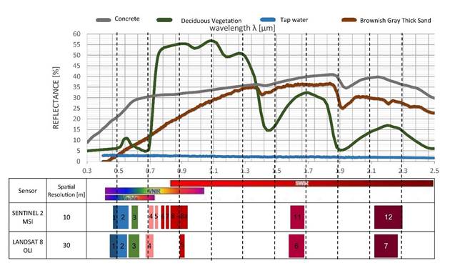
Figure 2 Spectral comparison of sensors L8 and S2 to determine LC. Developed by the authors with information from Baldridge et al. (2009), ESA (2013a), ESA (2013b), and USGS (2016).
Processing and Evaluation of the LC Classification
Table 2 shows the OA of all the algorithm-sensor combinations for each of the regions, in order of high to low. Region BG had the highest average OA for all the classifications (70.3 %), while BB resulted in 61.5 %, and VM in 58.2 %. The size of the area selected for each region may be a factor of influence, given that the highest OA corresponds to the area of analysis that is smallest in size. In BG, the water bodies cover a large area, which could have influenced the high OA obtained since an extra band helped to identify them using optic sensors and radar images are useful to detect water. In the case of the VM, the dynamics of change and the complexity of the area may have influenced the OA obtained for that region, which had the lowest average of the study regions. The bottom of Table 2 shows the results for each sensor. L8 presented the highest average OA, with 76.1 %, even though it had the lowest SR. That gives it the distinction of being a very useful sensor for defining LC types as well as other biophysical parameters. The performance of S2 was similar, with an OA of 75 %. S1 resulted in an OA of 38.8 %, which is much lower than the sensors mentioned above. The sensors that had the highest OA were those with the highest SpR. The low accuracy found with S1 may be due to the use of only three bands for the classification, which strongly differs from a report by Abdikan et al. (2016), who obtained the best results with the combination of bands VV, VH, and the subtraction of VV-VH. The MD was the classifier with the best performance, with an OA of 71.2 %, followed by SVM with 70.5 %, and SAM with 60.9%. The poorest performance was ML, with 50.7 %.
Table 2 OA of the LC classification for each sensor- algorithm combination implemented in this study.
| BB | BG | VM | ||||||
|---|---|---|---|---|---|---|---|---|
| Sensor | Algthm* | OA (%) | Sensor | Algthm* | OA (%) | Sensor | Algthm* | OA (%) |
| S2 | MD | 83.5 | L8 | SVM | 90.5 | L8 | SAM | 84.6 |
| S2 | SVM | 81.5 | L8 | ML | 88.6 | L8 | MD | 83.8 |
| S2 | SAM | 80.8 | S2 | SVM | 87.9 | L8 | SVM | 80.1 |
| L8 | SVM | 78.2 | S2 | MD | 86.2 | L8 | ML | 79.4 |
| S2 | ML | 77.4 | L8 | SAM | 86.1 | S2 | SAM | 71.5 |
| L8 | MD | 76.9 | S2 | SAM | 84.2 | S2 | MD | 67 |
| S1 | SVM | 68.6 | S2 | ML | 84.1 | S2 | SVM | 57.3 |
| S1 | MD | 62.3 | L8 | MD | 81.5 | S1 | MD | 46 |
| L8 | SAM | 57.9 | S1 | MD | 53.7 | S1 | SVM | 41.6 |
| S1 | SAM | 26 | S1 | SVM | 48.7 | S2 | ML | 39.2 |
| L8 | ML | 26 | S1 | SAM | 28 | S1 | SAM | 27 |
| S1 | ML | 18 | S1 | ML | 23 | S1 | ML | 21 |
| Average BB = 61.5 | Average BG = 70.3 | Average VM = 58.2 | ||||||
| Average by Sensor | Average by algorithm | |||||||
| L8 = 76.1 | S2 = 75 | S1 = 38.8 | MD = 71.2 | SVM = 70.5 | SAM = 60.9 | ML = 50.7 | ||
*Algthm: algorithm.
For the BB region, eight combinations had an OA over 60 %. The higher OA in this region was obtained with S2 combined with MD, SVM, and SAM (in that order), and the lowest OA was obtained with ML combined with L8 and S1 sensors. Based on these results, S2 is recommended for regions that are similar to BB (little precipitation and a large presence of irrigated cropland). The SR of S2 facilitates the identification of small objects of interest and was therefore helpful for this region, which contains large territorial contrasts.
For the BG region, eight combinations had an OA over 80 %: L8 and S2 combined with the four algorithms. The highest OA was 90.5 %, which was obtained with L8-SVM which presented the best performance of all combinations in this study. S2 with MD ended up in fourth place overall, even though its average OA was higher than those of the other algorithms. In contrast, the ML for this region had the second-highest OA, although it performed poorly in other combinations. The BG images have 1 to 3 % cloud cover, and images without clouds could not be found for that date. In addition, cloud cover and their shadows presented the highest accuracy in this region, which positively affected overall performance. Normally, S1 is advantageous for regions such as BG, where there is high precipitation and cloud cover since its technology is insensitive to those factors. However, in our case, this advantage did not mean improvements in the OA and this may be related to the fact that the selected images presented the above-mentioned percentages of cloudiness.
For the VM region, six combinations had an OA of over 60 %. L8 combined with the four algorithms resulted in the highest OA, even though more bands were used with S2. This indicates that this combination is suitable for regions with spatial configurations that are similar to VM (predominantly urban). This combination presented higher OA with SAM and MD. The OA was less than 60 % for S2 combined with SVM and ML. In this region, the results were poorest for S1-ML, S1-SAM, and S2-ML.
Figure 3 presents (in % of the domain) the presence of cover (PC), represented by a black square. AC (green bars), OC (red bars), and CC (blue bars) for the classifications with the best performance in each region are shown in the same figure. For BB, cropland-pasture presented the highest PrC (55.7) and AC (51.4) with the S2-MD combination. AC for human settlements was 3.0. For this category, CC was greater than OC, which indicates that this category was overestimated. Xerophytic mesquite and thorny shrubs have very similar spectral signatures, which resulted in high OO and CC values. The errors for bare soil may be due to confusion with areas where crops had been recently planted. Thus, a high number of pixels was mistakenly assigned to bare soil (1.8 of CC), and the category was overestimated. For BG, bare soil was the land cover with the lowest AC and PC, with 1.1 % in both values. The CC for cropland-pasture (0.9) and flood prone zones (2.5) may be due to their having very similar spectral signatures when crops begin to grow in those areas. Mangroves were distinguishable in the image and had a high AC (13 % for 15.5 % of PC). Water bodies had a low CC (0.1 %) since there was virtually no spectral confusion. Human settlements were underestimated, since CC for this class was lower than OC, with a PC of 2.8 %.
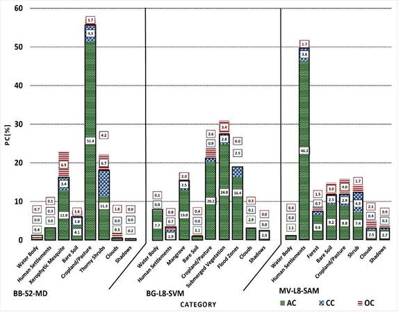
In the VM, urban zones were dominant, and the AC was high (46.3 % with a PC of 49.9 %), and they were correctly classified by the L8-SAM combination. Bare soil, forest, and water bodies had lower AC and PC. Cropland-pasture and shrubs had a low PC. For these cases, AC exceeded half of the PC. As in the other regions, OC was higher for bare soil and cropland-pasture, and the latter was confused with the shrub. Shrub and urban areas were overestimated, with a CC of 4.9 and 3.6 %, respectively. The remaining classes were underestimated, as indicated by an OC less than CC.
In all of the study regions, the dominant class made it possible to identify training areas with a high number of pixels and a homogenous spectral signature, resulting in high AC values. This proportional relation between PC and AC was reflected by bare soil, which had a low PC and AC. While shadows and clouds resulted in high AC levels, they do not contribute to the RC value, and furthermore, they make it difficult to adequately determine RC by making it difficult to identify the LC on the site.
Table 3 presents the PC results from the sensor-classifier combinations for the three regions. The combinations with the highest OA are highlighted in bold (S2-MD-BB, L8-SVM-BG, and L8-SAM-VM). For BB, L8-SVM and S1-SVM were the combinations with PC that were most similar to the one with the highest AC. The combinations with PC that were least similar to those with the highest AC were L8-ML and S1-ML. S1-SAM and S1-MD are not recommended because they overestimated or underestimated one of the classes studied.
Table 3 PC results, per category, for the sensor-classifier combinations, applied to regions BB, BG, and VM (in % of the domain)
| PC per category (see the meaning of numbers below the table) | ||||||||||||||
|---|---|---|---|---|---|---|---|---|---|---|---|---|---|---|
| 1 | 2 | 3 | 4 | 5 | 6 | 7 | 8 | 9 | 10 | 11 | 12 | 13 | ||
| Sensor/ Algorithm | BB | |||||||||||||
| L8 | MD | 0.61 | 4.39 | 21.93 | 6.21 | 49.1 | 16.81 | 0.37 | 0.59 | - | - | - | - | - |
| SAM | 0.45 | 4.04 | 24.29 | 6.96 | 41.56 | 20.37 | 0.5 | 1.84 | - | - | - | - | - | |
| ML | 0.42 | 4.92 | 19.64 | 55.7 | 17.71 | 0 | 1.09 | 0.53 | - | - | - | - | - | |
| SVM | 0.66 | 3.8 | 20.6 | 5.8 | 50.64 | 16.34 | 1.47 | 0.69 | - | - | - | - | - | |
| S1 | MD | 34.2 | 2.93 | 11.01 | 16.4 | 25.46 | 10.09 | - | - | - | - | - | - | - |
| SAM | 15.2 | 17.3 | 14.9 | 17.4 | 23.58 | 11.62 | - | - | - | - | - | - | - | |
| ML | 0 | 0 | 0 | 100 | 0 | 0 | - | - | - | - | - | - | - | |
| SVM | 0.89 | 2.3 | 20.25 | 4.78 | 44.81 | 26.96 | - | - | - | - | - | - | - | |
| S2 | MD | 0.4 | 3.3 | 16.23 | 5.92 | 55.64 | 17.93 | 0.36 | 0.21 | - | - | - | - | - |
| SAM | 0.42 | 2.78 | 19.65 | 6.22 | 46.4 | 21.74 | 0.58 | 2.22 | - | - | - | - | - | |
| ML | 0 | 8.54 | 30.96 | 4.09 | 55.87 | 0 | 0.38 | 0.15 | - | - | - | - | - | |
| SVM | 0.27 | 3.65 | 27.73 | 4.3 | 51.63 | 11.51 | 0.65 | 0.26 | - | - | - | - | - | |
| BG | ||||||||||||||
| L8 | MD | 7.58 | 2.31 | - | 2.74 | 17.77 | - | 1.3 | 1.73 | 18.2 | 29.9 | 18.5 | - | - |
| SAM | 9.29 | 1.51 | - | 1.76 | 21.07 | - | 1.73 | 4.73 | 17.7 | 26.7 | 15.5 | - | - | |
| ML | 7.03 | 8.9 | - | 3.62 | 20.48 | - | 4.73 | 1.78 | 14.2 | 23 | 16.3 | - | - | |
| SVM | 7.69 | 2.64 | - | 1.08 | 21.12 | - | 2.99 | 2.51 | 15.5 | 27.5 | 18.9 | - | - | |
| S1 | MD | 6.99 | 14.7 | - | 10.2 | 14.32 | - | - | - | 15.2 | 19.7 | 18.9 | - | - |
| SAM | 11.3 | 13.7 | - | 9.39 | 12.64 | - | - | - | 20.3 | 14.2 | 18.6 | - | - | |
| ML | - | 4.14 | - | - | 57.3 | - | - | - | - | 38.6 | - | - | - | |
| SVM | 8.23 | 1.56 | - | 20.5 | 24.97 | - | - | - | 28 | - | 16.7 | - | - | |
| S2 | MD | 7.83 | 1.14 | - | 1.55 | 22.25 | - | - | - | 18.6 | 27.6 | 21 | - | - |
| SAM | 8.29 | 0.77 | - | 1.12 | 18.62 | - | - | - | 15.9 | 34 | 21.3 | - | - | |
| ML | 7.84 | 6.05 | - | 5.77 | 22.56 | - | - | - | 16.2 | 23.6 | 18 | - | - | |
| SVM | 7.97 | 3.95 | - | 3.64 | 20.61 | - | - | - | 19.4 | 26.9 | 17.5 | - | - | |
| VM | ||||||||||||||
| L8 | MD | 1.21 | 50.5 | - | 13 | 17 | - | 2.67 | 0.91 | - | - | - | 5.68 | 9.04 |
| SAM | 1.1 | 49.9 | - | 11.8 | 11.77 | - | 2.92 | 3 | - | - | - | 7.29 | 12.3 | |
| ML | 1.11 | 58.8 | - | 6.67 | 16.86 | - | 1.68 | 1.01 | - | - | - | 4.6 | 9.32 | |
| SVM | 2 | 59.3 | - | 6.49 | 14.57 | - | 3.3 | 1.22 | - | - | - | 5.16 | 7.97 | |
| S1 | MD | 2.27 | 35.8 | - | 10.5 | 13.96 | - | - | - | - | - | - | 24.3 | 13.2 |
| SAM | 20.6 | 31.1 | - | 17.4 | 12.73 | - | - | - | - | - | - | 10.1 | 8.19 | |
| ML | 2.08 | 0 | - | 0 | 0 | - | - | - | - | - | - | 0 | 97.9 | |
| SVM | 2.1 | 51.4 | - | 9.86 | 12.1 | - | - | - | - | - | - | 8.85 | 15.7 | |
| S2 | MD | 2.09 | 45.3 | - | 12.3 | 23.92 | - | 1.07 | 0.91 | - | - | - | 6.64 | 7.83 |
| SAM | 1.06 | 43 | - | 14.4 | 20.39 | - | 3.25 | 2.94 | - | - | - | 5.41 | 9.64 | |
| ML | 0.88 | 46.9 | - | 25 | 8.57 | - | 0.77 | 0 | - | - | - | 16.7 | 1.16 | |
| SVM | 0.88 | 45.5 | - | 7.15 | 13.37 | - | 0.97 | 20.2 | - | - | - | 4.26 | 7.69 | |
1 = water bodies; 2 = human settlements; 3 = bare soil; 4 = cropland-pasture; 5 = cloud cover; 6 = shadows; 7 = xerophytic mesquite; 8 = thorny shrubs; 9 = mangroves; 10 = submerged vegetation; 11 = flood prone zones; 12 = forest; 13 = shrub.
For the BG region, the PC obtained with S2-SVM and S2-MD were similar to those obtained with L8-SVM (which had the highest OA). The combinations that overestimated or underestimated PC were all the combinations with S1. As previously observed, using S1 for regions similar to BG (humid tropical) with cloudy conditions less than 3 % would result in considerable errors that would need to be corrected. Frequent cloud cover significantly reduces the ability to use optical images and according to our findings, these should be occupied with cloud cover less than 3 %. Additionally, we do not recommend the L8-ML combination to study human settlements in regions similar to BG, since that would overestimate PC.
For the VM region, the PC obtained with L8-SAM was comparable to S1-SVM and S2-SAM. The combinations that differed the most from what was obtained with L8-SAM were S1-SAM, S1-MD, and S2-ML, and therefore, they are not recommended. The PC obtained with L8 was similar to all the algorithms tested, which is a strong argument for recommending the use of this sensor with any of the classifiers for regions where urban land cover is predominant.
Calculation of RC
Table 4 shows the factors that this study took into account to select the most useful image for calculating RC: start of the study period, TR, SR, SpR, and Sensitivity to weather conditions. At the bottom of the table, the obtained average OA by the sensor is included as a reference. The TR of S2 (five days) was better than that of L8 (16 days) and S1 (12 days). S2 began to acquire images in 2015 and L8 in 2012. L8 can be complemented with the Landsat series, which has been available since 1972. S1 images have been available for all of Mexico since 2016. While S1 and S2 have the disadvantage of being only recently launched their SR is higher than that of L8 which makes it possible to distinguish LC having a small presence. For example, in BB, the SR of S2 made it possible to classify areas that had high contrast and covered a small area. Nevertheless, the size of the studied hydrological region should be considered, since a high SR requires a longer processing time and higher computing capacity.
Table 4 Factors for selecting an image for the determination of LC to obtain RC.
| Sensor | |||
|---|---|---|---|
| Factor | L8 OLI | S1 SAR | S2 MSI |
| Start of the study period of the research to be performed | 1972* | 2016 | 2015 |
| Suitable for studies | Historical | Current | Current |
| TR [d] | 16 | 16 | 5 |
| Suitable for studies | Every two weeks | Every two weeks | Weekly |
| SR [m] | 30 | 10 | 10 |
| Suitable for studies | Regional/Local | Regional/Local | Regional/Local |
| SpR range [µm] | 0.48-2.2 | 37 500-75 000 | 0.44-2.19 |
| Suitable for LC type | Water bodies, vegetation, bare soil, and human settlements | Water bodies, vegetation, bare soil, and human settlements | Water bodies, vegetation, bare soil, and human settlements |
| Sensitivity to weather conditions | Yes | No | Yes |
| Suitable for studies | Regions with little cloud cover | Regions with large cloud cover | Regions with little cloud cover |
| (%) Average OA in the present study | 76.10 | 38.75 | 75.04 |
All three sensors were able to distinguish the four main LC categories in the study: water, bare soil, human settlements, and vegetation. The greater number of bands in S2 did not result in a higher OA. Also, the three bands in S1 did not provide good classification results. Although this sensor is associated with the good classification of urban areas with a high SR (Goldewijk, 2001; Liu & Tian, 2010; Loperfido, Noe, Jarnagin, & Hogan, 2014), its use in the present study did not improve the results in the VM region (highly urbanized). Given the TR of the sensors used in this study, any one of them could be used to perform the analysis presented by this investigation. S1 can be used with high cloud cover, in which case it will be helpful to use the combinations that the previous section indicated as having the highest accuracy. Certain actions are recommended to improve the classification results, such as post-processing techniques, increasing the number of bands, and selecting training areas that have a larger number of pixels and spectral homogeneity (Congedo, 2016; Richards & Xiuping, 2013; Chuvieco, 1991). Table 4 can be used as a reference for selecting the image. Data from S1 and S2 can be used if the project being conducted involves the study of current LC, but if the study includes historical changes it will be limited to the data from the Landsat series, which has generated images since 1972. All three sensors can be used for regional or local analyses, and enable identifying water bodies, vegetation, bare soil, and human settlements with a good degree of accuracy. After consulting Table 4 to select the most suitable sensor, we recommend that it be combined with the algorithm having the highest degree of accuracy, as reported by this study’s findings (Table 2).
Figure 4 shows the RC results for each region, including the LC classification obtained with the sensor-algorithm combination having the highest OA, and four geographic layers: MP, ST, the resulting RC, and the RC from INEGI (2010) (official information) for comparison purposes. The following observations are applicable to all the study areas. The spatial distribution of the RC obtained by the present study is drastically different than those from INEGI’s hydrological chart, 2010. The information presented in the INEGI layers is much more general than the layers that resulted from our study. The information resulting from our study has a higher SR (10 m). In the case of INEGI, the data are at a scale of 1:50 000. INEGI’s RC values were not determined in a precise manner, but rather, there are five discrete categories, the highest of which is between 0.10 and 0.20 for BB and VM, and ≥ 0.3 for BG.
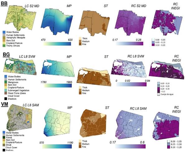
Figure 4 LC classifications were obtained with the sensor-algorithm combination having the highest OA and the layers MP, TS, resulting RC, and the RC from INEGI (official information), for the three regions studied.
In the case of BB, the combination that was selected was S2-MD. MP ranged from 470 to 620 mm and increased towards the southern portion of the hydrological region. The dominant ST was medium, with small areas of fine texture and very little thick texture in the north. The RC ranged from 0.17 to 0.28, with the latter exceeding the upper limit reported by INEGI (0.20). The spatial distribution was quite different from INEGI’s hydrological chart. The RC in the chart ranged from 0 to 0.5 % in the southeast and north, while our study resulted in a smaller RC for a larger area of the northern portion of the region. In our study, the highest values were found in the south, whereas the INEGI chart identified the northwest as having the highest values.
For the BG region, the LC was obtained with L8-SVM. The lowest MP was 1 780 mm, which increased to nearly 2 000 mm towards the west. The dominant ST was fine, medium in the south, and thick in the north. The RC ranged from 0 to 1, with a predominance of values over 0.85. The highest RC values were in the western portion of the hydrological region, whereas the INEGI chart identified the central region as having the highest values.
For the VM region, LC was obtained with the L8-SAM combination. The minimum MP was 570 mm, which increased to 1 190 mm towards the west. The dominant ST was fine, with the medium in the central region and thick in the northeast. The RC ranged from 0.17 to 0.6, with a predominance of values over 0.24. The highest values were found in the central portion of the region, which may be because the calculation used by the present study included MP as a variable that is important to the RC value, considering that an immediate relationship between the two can be seen when visually comparing the RC results with the MP map.
Conclusions
This study presents findings and recommendations for selecting open-access satellite images to calculate LC and RC based on the conditions of the study area. Nevertheless, the results and recommendations are applicable to any study that uses these types of images to determine LC. In our particular case, the characteristics of the sensors analyzed made it possible to obtain LC, which was needed to determine the RC for the study area. Different results were obtained with each one of the sensors. For the determination of LC, sensor L8 had the highest OA, on average, followed closely by S2, while S1 had the lowest values. Based on this study, the determination of LC should prioritize the use of MD and SVM, and avoid ML. This is an important finding given that ML is typically considered to be a standard algorithm and the first choice. Concerning SAM, this can be used in areas with characteristics that are similar to VM.
High SR is helpful for determining LC in areas such as the BB region (semi-arid with a large amount of irrigated cropland and isolated human settlements). As a result, the best accuracies were obtained with S2. The recommendation for regions that are similar to BB is to combine MD, SVM, and SAM with S2. ML should be avoided for this type of region. The LC for BB presented a high CC for xerophytic mesquite-thorny shrub and cropland-bare soil. We recommend that training areas for water bodies be carefully determined, given that they have a small presence in regions such as BB. Cropland-pasture is dominant in these regions, while water bodies and human settlements are scarce. For the BG region, L8-SVM had the highest OA. The use of the deep blue band seemed to indicate an improvement in the AC obtained from the determination of water bodies. In regions with climates that are similar to that of BG (high cloud cover and precipitation), the use of S1 with MD and SVM is an option, with the largest possible number of bands and post-processing techniques. Even though this has resulted in inaccuracies of 50 %, which can be explained by having occupied images with little cloud cover (< 3 %), it would not otherwise be possible to conduct studies with optical images, and with more cloudy conditions the results should improve. In this type of region, submerged vegetation, cropland-pasture, and flood-prone zones have the largest PC, while bare soil and human settlements have the smallest. Since L8-SAM was the best combination for the VM region, we recommend this option for similar regions (temperate climates with a predominance of urban zones). S2 is also recommendable. The use of S1 and the ML algorithm should be avoided in these regions.
The selection of the ideal image for determining LC is a decision that should take into account the following factors: availability, TR, SR, SpR, study period, LC type and its dynamic, climate, and size of the study area. These should consider the following:
Historical availability of data with TR: the Landsat series is useful for long-term analyses, and S1 and S2 for current analyses.
Periodicity of the analysis for TR: S2 is useful for weekly studies and the other three sensors for longer periods.
The scale of the project and SR: all of the sensors that were studied function for regional and local projects.
Type of LC and spectral bands (SpR). The sensors studied are capable of distinguishing the four groups that are determinants of RC: water, bare soil, human settlements, and vegetation. For other classes, we recommend performing the analysis of bands that were presented in this study.
Only radar sensors can be used for regions with high cloud cover, in spite of the low OA found in our study.
By using this method to determine RC, accurate and updated values were obtained with a resolution of up to 10 m, on a continuous scale. This represents an advantage over the official information in countries such as Mexico whose INEGI’s hydrological chart groups regions into classes with values from 0 to 5 %, from 5 to 10 %, etc. The use of the RC maps obtained by this study will improve both the results from spatial hydrology analyses and the process for making spatially differentiated decisions.

