


 nueva página del texto (beta)
 Inglés (pdf)
 Artículo en XML
 Referencias del artículo
 Enviar artículo por email
 Citado por SciELO
  Similares en
SciELO
Similares en
SciELO 
 Permalink
Introduction
Flash floods are defined as floods that occur over a short period, and usually carry a significant amount of debris. They can be observed mostly in streams with high longitudinal slopes; however, the phenomena can also take place when sediment is rapidly transported as a result of heavy rainfalls (Ballesteros-Cánovas et al., 2011). Authorities, practitioners and researchers, need to know the discharge of flash floods in order to propose better water and flood risk management plans. Yet, direct measurement of peak flash flood discharges is challenging owing to the flood’s destructive nature (Bull & Kirkby, 2002) and the inability to provide reliable rating curves for high-magnitude flows. Indirect peak discharge estimates are thus considered to be a more practical alternative.
As part of the indirect methods, hydraulic modelling is perhaps the most common approach. It can be used to estimate peak discharge if sufficient observations or records of the peak water flow height are available (Herschy, 1998; Simmers & IAH, 2003). However, there are issues associated with the errors of conventional one-dimensional (1D) hydraulic estimates. Slope-area methods, for instance, can overestimate discharge by up to 50 % (Lumbroso & Gaume, 2012), and by more than 100 % in rivers with steep slopes (more than 0.01 m m-1).
Given the limitations of these existing methods, two-dimensional (2D) hydraulic modelling is now regarded as a better choice. It avoids the subjectivity of 1D modelling, in which representative channel cross-sections have to be chosen from an often quite variable river reach (Hunter, Bates, Horritt, & Wilson, 2007). Conversely, 2D modelling requires a Digital Elevation Model (DEM), and thus the characteristics of the river bed are better represented, and a more accurate estimation of discharge can be expected where high-resolution DEMs are available. However, in developing countries such as Ecuador, high-resolution DEMs are less widely available than in more developed countries. The solution to this issue might be provided by photogrammetric techniques.
Finally, video recordings of flood events are commonly found nowadays online, providing an opportunity to gain more information on the flood events and assist discharge estimates.
This study’s aim is to explore the use of an ensemble composed of 2D hydraulic modelling, together with Structure-from-Motion (SFM) and YouTube videos to obtain reliable post-flood, indirect estimates of peak discharge for an ephemeral river. This aim will be achieved through the following specific objectives:
Obtain a sub-metre-resolution DEM of the river reach using SfM techniques;
Employ YouTube videos to estimate “observed” high water marks/levels and water velocity; and,
Incorporate this data into a state-of-the-art 2D hydraulic model and perform several 2D hydraulic simulations to find the best fit with the “observed” parameters.
Study area
Manta city region in coastal Ecuador is often affected by heavy, many of which resulting from El Niño (ENSO). In 2012, 300 dwellings were affected and 40 persons were displaced from their homes as a result of flash floods in the Burro River (El Universo, 2012; El Diario, 2012). This river has flooded several times, and inhabitants know they are at risk when heavy rains occur (El Diario, 2016). Despite these issues, to date, local authorities do not have publicly available estimates of the volumes of water flowing in this river during flash flood events.
The catchment of Burro River is located in a semi-arid region (Giler-Ormaza, 2018) which is heavily urbanized. GIS analysis based on online Ecuadorian Government data suggests that 14.7 % of the catchment area upstream of the study reach is an urban zone. However, based on field recognition, we estimate a larger proportion of the land use to be an urban zone.
One reach for Burro River has been selected. This particular reach was chosen because of the availability of video recordings on YouTube, which allows for better indirect flood estimation. It will hereafter be referred to as the “Burro reach” (WGS84 17S coordinates S 9893400; W 532000) and has an upslope drainage area of 32.38 km2. Reach length is ~110 m, but width varies between 17 and 22 m. There are two sections of the Burro reach, divided by a bridge (Figure 1). The width of the reach (including its banks) upstream of the bridge (sub reach BU) is 17 m, while downstream from the bridge (sub reach BD) the width is 22 m. The river bed is covered with naturally growing weeds with banks protected with gabions. The local soil is highly erodible.
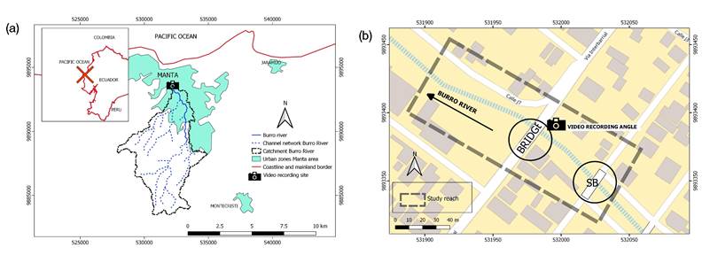
Figure 1 (a) Burro River Study Area. Location in Ecuador and Burro river catchment in Manta city; (b) “Burro reach” and its urban surroundings at flood risk are shown. Water flows from the bottom right to the top left. Note the bridge in the middle of the reach and also the “smaller bridge” (SB) located immediately upstream of the reach. The angle from which the YouTube video was recorded is also represented.
At the time of data collection for this study, the Burro reach was densely vegetated, which poses a challenge to the SfM technique and the indirect peak discharge estimate.
Materials and methods
DEM creation
Since Smith, Carrivick, Hooke and Kirkby (2014) established that SfM provides a high accuracy DEM when compared to dGPS surveyed cross-sections, no cross-sections were surveyed, and only a SfM survey was carried out. Highly visible targets (400 mm in height) were deployed across the study reach as Ground Control Points (GCPs) to overcome the widespread presence of vegetation in the river reach. Since the study rationale was to use only commonly available equipment and methods suited for use in the developing world, a compass bearing and a low-cost Laser Rangefinder (LRF) Nikon 550 AS were employed to survey the GCPs in a local coordinate system. The LRF is believed to suffice for this type of data collection since it is accurate to the decimeter level (Smith et al., 2014). With an accuracy of this level, the resulting point cloud will allow for the 2D hydraulic modelling to be performed with sufficient accuracy, given the application for which it is being employed.
Photographs of the Burro reach were taken from the highest points of the nearby banks and bridges (Figure 2) with a commercial camera (NIKON COOLPIX S3400). The reach was divided into two sections: one section upstream of the bridge (hereafter called BU) and another downstream from the bridge (hereafter called BD).
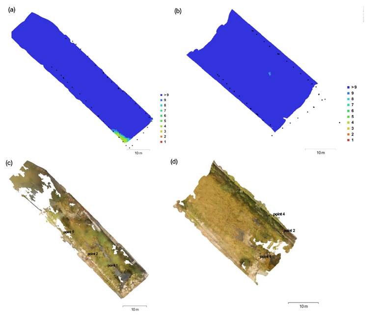
Figure 2 Plan view with details of the fieldwork for the sections surveyed: a) show the camera locations (black dots) and the image overlap (coloured scale) for (a) Burro Upstream (BU) and (b) Burro Downstream (BD) section. Note the semi-loop followed to take the pictures and the almost uniform overlap for all surveys. (c) and (d) are the plan view with details of the fieldwork for the sections surveyed for BU section and BD section respectively. The water flows from the bottom right to the top left.
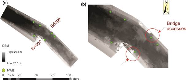
Six GCPs were laid for the Burro reach, three at each side of the bridge. While more GCPs and a greater spatial distribution would have been preferable, Smith et al. (2014) found good results with few GCPs; however, the same study found that the SfM-generated point cloud deviated from the actual terrain elevation for those points located far from the GCPs. High water marks are ideally surveyed directly during fieldwork; however, this proved impractical because the flash flood event studied took place several years ago, and there were no remaining high water marks in the selected river reach. On the other hand, the availability of video recordings allowed for the recognition of high water elevations (HWE).
Amongst alternatives for SfM processing, such as 123D Catch (Autodesk, 2016) and Photomodeler (Photomodeler, 2016), Agisoft PhotoScan was chosen to build the point cloud. This software provides a Graphical User Interface (GUI) in which both SfM and MVS can be found (Agisoft, 2016). The GUI provided an easy-to-follow workflow which guides the user through the necessary steps. The photographs were aligned and the GCPs were manually identified. Agisoft allows for the evaluation of the errors between the GCPs local coordinates and the point cloud coordinates assigned by the software.
The resulting dense point cloud was exported for further processing to the free/open-source software CloudCompare (CC) (Girardeau-Montaut et al., n.d.). Burro reach sections were merged manually in CloudCompare by aligning the clouds using easily identifiable common points. The point clouds were then Octree resampled to decimate the dense Agisoft output, reducing the number of points between ten and one-hundred thousand, which is necessary for creating a bathymetry for 2D hydraulic modelling. Finally, DEMs were transferred to ArcMap for further analysis and visualization (Figure 3).
High water marks (elevation) and water velocity measurements from YouTube
The use of YouTube videos to inform hydraulic modelling is relatively novel; nonetheless, it has shown considerable promise (Le-Boursicaud, Pénard, Hauet, Thollet, & Le-Coz, 2016). This type of approach allows for a more complete assessment of flash flood peak discharges because velocity values can also be inferred from the videos. Another advantage of using YouTube videos is the emerging concept of “citizen science” (Buytaert et al., 2014) in hydrologic research. This can allow researchers and practitioners to obtain more evidence to strengthen their analyses of peak discharge and related events. Video recordings could thus be a good and innovative alternative approach to the identification of high water marks.
The video of the Burro river reach can be found on the YouTube platform (https://www.youtube.com/watch?v=QPEYdHd_8DY). The video was not recorded by the authors of this paper. Attempts were made to contact the video’s owner, without success. From the video, High Water Elevation (HWE) points were inferred for the Burro reach, and as were surface water velocity estimates. HWE marks are useful to compare and calibrate the hydraulic modelling outputs. For HWE points, visual identification focused on points that are readily found in the video, point cloud and DEM. This led to the choice of HWE in the bridge accesses used for maintenance (hereafter simply called bridge accesses) and in the first row of gabions of the right river bank. As a basic rule, the hydraulic simulations are intended to comply with the condition of not flooding the “bridge accesses,” as can be observed in the corresponding video. For these reasons, HWE marks were placed around that area (Figure 3).
For water velocity measurements, two images from the video, in which a floating object appears, the distance that the object has travelled (through a control section) and the time of travel were employed to compute the water surface velocity. The latter result is used with a coefficient to transform water surface velocity to depth-averaged velocity. Following Dramais, Le-Coz, Camenen and Hauet (2011), the coefficient was set to 0.8. By having one single depth-averaged velocity value, this approach enables the assessment of the 2D hydraulic modelling results. Confirmation of the velocity was carried out using the velocity-head method (see equation 1) on the piers of a smaller bridge (SB) located just upstream of the Burro reach (See Figure 1). In this paper, said velocity is referred to as “observed” velocity.
The velocity-head method computes velocity (v, in m s-1) based on the difference in water surface elevation (Δh, in m) between the upstream and the downstream of an obstacle and the acceleration due to gravity (g, in m s-2). These are employed in Bernoulli’s equation, assuming the water velocity immediately upstream from the obstacle to be zero.
Hydraulic modelling
Rapid initial estimation of flow rate
The Slope-conveyance method was briefly employed as a guide for the input discharges to be modelled by the 2D modelling software. The wetted perimeter and wetted cross-sectional area were computed based on the HWE points from the video recordings. The Manning’s n value chosen was 0.06, based on tables provided by Arcement and Schneider (1989), and Chow, Maidment and Mays (1988).
2D hydraulic modelling
Hydraulic modelling in 2D was undertaken instead of 1D modelling, following the consideration of several aspects. First, river flows can be considered a dynamic process and conveyance capacity should not be determined by taking into account only one cross-section. Instead, a river reach should be considered (Guan, Carrivick, Wright, Sleigh, & Staines, 2016). 2D hydraulic modelling allows for a visual evaluation of different localized events of critical importance, such as high localized velocities. Many localized events may be found in a single reach, given that vegetation cover and river bed elevation are spatially variable throughout the reach. Spatially distributed visualization of the interactions between river bed and flow can be obtained with 2D hydraulic modelling. Furthermore, concerning our study reach, which is surrounded by bridges and located in an urban area, 2D hydraulic models might be better suited to represent the velocity (Gaume & Borga 2008). Among the different 2D modelling suite options available, Delft3d was chosen. This software now has a free/open-source version, has performed well in hydrodynamic simulations (Williams et al., 2013; Yuill, Gaweesh, Allison, & Meselhe, 2016; Gebrehiwot, Haile, De-Fraiture, Chukalla, & Embaye, 2015; Hosseini & Coonrod, 2011), and has already been used in conjunction with SfM (Javernick, Hicks, Measures, Caruso, & Brasington, 2016; Smith et al., 2014).
Delft3d comprises several modules for different applications. For this study’s purposes, only three components were necessary: RGFGRID, QUICKIN and FLOW. The point cloud created in Agisoft and edited in Cloud Compare is imported as a “sample” in RGFGRID and a grid is created. The grid was created with less than 0.02 orthogonality to comply with the condition of the Delft3d FLOW module (Deltares, 2014). The mean grid cell size is less than 0.25 m2. As with other 2D modelling suites, if the cell size were smaller, the required processing time would increase significantly (Néelz & Pender, 2013). Because several runs were attempted in this study, and sensitivity analysis for certain parameters was performed, long processing times were not desired.
Moving to QUICKIN, a depth map (i.e., bathymetry) is created within Delft3d. The options employed are Grid Cell Averaging, Triangular Interpolation and Internal Diffusion. For more details on the functioning of these options, the reader is referred to Deltares (2011). For the creation of the bathymetry, the corresponding point cloud created was used.
After a rapid sensitivity analysis of all parameters and from a review of the literature, the following combination of parameters was employed: a) the time step at 0.001 minutes; b) two “time-discharge” boundary conditions located at the upstream and downstream boundaries of the reach, which allowed us to constrain the modelling based on flow rate and time (i.e., a hydrograph); c) the roughness parameter was set at 0.06; d) the eddy viscosity at 0.01 m2/s; and e) the numerical “scheme” was set at “flood”. Roughness is harder to define for 2D modelling when compared to Manning’s n employed in 1D modelling since when using 2D models, part of the roughness is already explicitly represented by the digital terrain model (i.e., the bathymetry in Deflt3d). In addition, worldwide there is less experience using 2D modelling. It was finally decided that values from the tables of Arcement and Schneider (1989) and Chow et al. (1988) would be used, taking into account the extensiveness of vegetation cover.
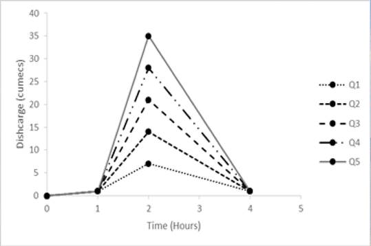
The simulations are intended to comply with the condition of not flooding the “bridge accesses” as observed in the video. Input hydrographs (presented in Figure 4) were adopted based on the rapid slope-conveyance computation employed to approach reasonable discharge values. The validity of these values was also confirmed following analysis of flow envelope curves, as suggested by Lumbroso and Gaume (2012).
To quantify vertical errors in the simulations, three metrics of residuals were selected. Those were the Root Mean Squared Error (RMSE), the Mean Error (ME) and the Mean Absolute Error (MAE). The residuals were computed based on a comparison of the water depth observed (in the video) and modelled (with Delft3d).
In summary, several hydraulic simulations were performed in Delft3d. The three criteria that were employed to establish whether the peak discharge estimates can be considered reliable were: a) the vertical accuracy (residuals) of the HWE points; b) the inundation of the bridge accesses; and c) the water velocity. Additional criteria used was the accuracy of the estimates in x and y (from plan view); however, this was not quantified, but rather assessed only visually with the spatially distributed outputs of Delft3d. A diagram to summarize the methods is presented in Figure 5.

Results
Georeferencing errors in Agisoft were different for the upstream (RMSE = 0.17 m) and downstream (0.30 m) reaches; however, both are within the accuracy anticipated for the laser rangefinder method.
Six HWE points were selected for our study reach (see Figure 3 and Figure 6). Pointcloud editing in CC was undertaken to eliminate excessive vegetation in several areas of the reach, especially, dense vegetation patches in the area near the right-hand access to the bridge. Consequently, the final DEM and bathymetry do not adequately represent part of the right bank. Nevertheless, one HWE point was placed there to quantify the vertical error. If the video recordings for the Burro reach had been obtained from a higher position, more GCPs could have been used.
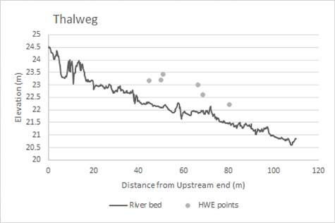
Figure 6 Long profile of Burro River reach bed at the thalweg. High water elevation (HWE) points are also shown.
The residuals are summarized and presented in Table 1. Many are smaller than the Delft3d grid cell size, and the best fit is similar to the point cloud georeferencing error (0.30 m). However, not accounting for horizontal errors numerically can be considered a limitation. This limitation of the numerical assessment confirms the need for visual, spatially distributed results from Delft3d. The planform inundation maps confirm the findings presented in the residuals table.
Table 1 Metrics of residuals of simulations. RMSE is the Root Mean Squared Error, ME, the Mean Error; and MEA, the Mean Absolute Errors. The best fits are in bold.
| Discharge (m3 s-1) | Residuals | ||
|---|---|---|---|
| RMSE (m) | ME (m) | MAE (m) | |
| 7 | 0.57 | -0.51 | 0.51 |
| 14 | 0.43 | -0.28 | 0.34 |
| 21 | 0.50 | 0.08 | 0.46 |
| 28 | 0.59 | 0.27 | 0.53 |
| 35 | 0.65 | 0.40 | 0.60 |
The results shown in the distributed velocity output maps (Figure 9) are compared to the velocity estimates from the video (Figure 7). In Figure 9, the velocity in the middle of the river matches those estimates from the video (between 3 and 4 m3 s-1). This might suggest that 21 m3 s-1 is closer to being the actual discharge. However, in Figure 8, it is observed that with such a discharge (21 m3 s-1) there is 0.30 m of water depth in the left access of the bridge. Since the criteria are not in agreement, what could then be stated is that the actual discharge for the Burro reach is likely to be between 14 and 21 m3 s-1. Note that the increase in velocity in the zoomed-in area seems to correspond to a funnel effect caused by the vegetation patch near the right access of the bridge. Interestingly, it is possible that such an effect took place at the moment when the video was recorded. Finally, Froude numbers for the Burro reach (not presented) indicate patches where subcritical flow dominates and others where critical and supercritical flow occur. Most of the Froude number values fell within 1.3 and 0.8.
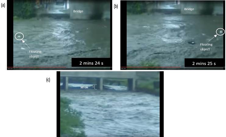
Figure 7 Key images for measurements from YouTube videos: (a) show the extent of the “control section” when a floating object enters, and (b) when it exits the section. The bridge access of the left bank can be observed. One of the HWE points was placed in that location. In (c) the section employed to apply the velocity-head method. Notice the jump in the piers of the smaller bridge (SB) located immediately upstream from the study reach.

Figure 8 2D hydraulic modelling results for water depth at the Burro reach. Water depth simulation results for (a) 7 m3/s; (b) 14 m3/s; (c) 21 m3/s; (d) 35 m3/s.

Discussion
The ensemble of 2D hydraulic modelling, SfM and YouTube videos has been shown to work well and provide estimates for the peak flow rate of a flash flood occurring in an ephemeral river.
Regarding fieldwork, SfM is a rapid and inexpensive tool to obtain DEMs (Carrivick, Smith, Quincey, & Carver, 2013), and while Smith et al. (2014) mentioned that the applicability of SfM techniques is limited to certain types of reaches, namely those with little standing water and scarce vegetation cover; here, the terrain model generated responded well to the 2D hydraulic modelling despite challenges with the extensive vegetation cover of the Burro reach. This study’s results thus seem to broaden the applicability of the SfM approach. The DEM obtained has a high resolution, especially for such a data-scarce area.
Considering velocity estimates, if the control section distance is short (in our case 5 m; see Figure 5 (a and b) errors in velocity estimates are likely to increase. Here, the availability of only one video recording limited the measurements. We believe low video resolution and short control sections are unlikely to be problematic in the near future since more video recordings could be available; especially if local authorities adopt the approach presented here and encourage people by the river to pro-actively take video footage of floods as a part of flood risk management.
Finally, compared to slope-conveyance or 1D hydraulic modelling, the 2D approach requires significantly more time to run and a higher level of user expertise. There are more ways in which the outputs of 2D modelling could be affected. Eddy viscosity values, the time step, grid resolution (i.e., cell size) and Courant numbers for numerical stability (Deltares, 2016) must be carefully handled. In the several iterations undertaken here, it was noted that when the time step was inadequate, unrealistic patterns of flow depths and flow directions emerged; leading to erroneous quantification of the most appropriate fits.
Conclusions
An ensemble of 2D hydraulic modelling software (Delft3d) together with SfM and YouTube videos was explored. To the authors’ knowledge, this the first time that such an ensemble has been tested. With this ensemble, estimates of peak discharge have been made for a flash flood event occurring in an ephemeral river. Several discharge simulations were tested to find the best fit with the “observed” parameters at 0.43 m (RMSE). For the flood event is shown in the video, the actual discharge for the Burro reach is estimated as being between 14 and 21 m3 s-1. From the simulations, some high-velocity patches (3 to 4 m s-1) match the “observed” velocities and lend support to the discharge values estimated using high water marks.
The ensemble can be developed into a powerful tool for indirect peak discharge estimates in ephemeral rivers There are clear benefits to using this workflow in developing countries, where resources are frequently limited. Looking further, the ensemble can become a tool of flood risk management specially in semi-arid and arid regions.

