


Servicios Personalizados
Revista
Articulo
 texto en
  Inglés (pdf)
 Artículo en XML
 Referencias del artículo
 Enviar artículo por email
Indicadores
-
 Citado por SciELO
 -
 Accesos
Links relacionados
-
 Similares en
SciELO
Similares en
SciELO
Compartir

 Permalink
Tecnología y ciencias del agua
versión On-line ISSN 2007-2422
Tecnol. cienc. agua vol.12 no.3 Jiutepec may./jun. 2021 Epub 26-Jun-2025
https://doi.org/10.24850/j-tyca-2021-03-02
Articles
Estimation of reference evapotranspiration from temperature data: A comparison between conventional calculation and artificial intelligence techniques in a warm-sub-humid region
1
 http://orcid.org/0000-0002-0921-7738
2
http://orcid.org/0000-0002-9356-6251
3
http://orcid.org/0000-0002-8018-7869
1Colegio de Postgraduados, Campus Campeche, Sihochac, Champotón, Campeche, México, l_ramos90@yahoo.com
2Colegio de Postgraduados, Campus Campeche, Sihochac, Champotón, Campeche, México, quej@colpos.mx
3Colegio de Postgraduados, Campus Campeche, Sihochac, Champotón, Campeche, México, ceugenio@colpos.mx
4Colegio de Postgraduados, Campus Campeche, Sihochac, Champotón, Campeche, México, evarardo.aceves@colpos.com
5Universidad Popular de la Chontalpa, Cárdenas, Tabasco, México, brivera@colpos.mx
Reference evapotranspiration (ETo) is an agro-meteorological parameter of great importance for many areas of study such as geotechnics, climatology and hydrology, where its greatest importance falls in the calculation of the crop’s evapotranspiration (ETc). In this study, using only temperature data, the performance of three artificial intelligence models and two conventional equations to predict the reference evapotranspiration (ETo) was evaluated in a warm sub-humid climate in México. The artificial intelligence models evaluated were: support vector machines (SVM), Gene Expression Programming (GEP) and XGBoost, and the conventional models were those by Hargreaves-Samani and Camargo. The performance of the models was evaluated according to the statistical indexes: Mean Absolute Error (MAE), Root Mean Square Error (RMSE), Coefficient of Determination (R2) and Mean Bias Error (MBE). Confidence intervals were constructed for each statistical index using the technique of bootstrap resampling with the purpose of evaluating their uncertainty. The results show that among the conventional models evaluated, the equation by Camargo obtained a better performance in the estimation of ETo compared to the equation by Hargreaves. Regarding the artificial intelligence models, the SVM model obtained the best performance among the techniques evaluated. In general, it is recommended to use the SVM model to estimate the ETo values since it outperforms the other techniques.
Keywords: Reference evapotranspiration; artificial intelligence techniques; automated weather stations; bootstrap
La evapotranspiración de referencia (ETo) es un parámetro agro-meteorológico de gran importancia para muchas áreas de estudio como la geotecnia, climatología e hidrología, donde su mayor importancia recae en el cálculo de la evapotranspiración de cultivo (ETc). En el presente estudio, utilizando solamente datos de temperatura, se evaluó el desempeño de tres modelos de inteligencia artificial y dos ecuaciones convencionales para predecir la evapotranspiración de referencia (ETo) en un clima cálido subhúmedo en México. Los modelos de inteligencia artificial evaluados fueron máquinas de soporte vectorial (SVM), programación de expresión genética (GEP) y XGBoost, así como los modelos convencionales de Hargreaves- Samani y Camargo. El desempeño de los modelos se evaluó de acuerdo con los índices estadísticos error absoluto medio (MAE); raíz cuadrada media del error (RMSE); coeficiente de determinación (R2), y el error medio de sesgo (MBE). Se construyeron intervalos de confianza para cada índice estadístico utilizando la técnica de remuestreo bootstrap, con el propósito de evaluar la incertidumbre de los mismos. Los resultados demuestran que entre los modelos convencionales evaluados la ecuación de Camargo obtuvo un mejor desempeño en la estimación de la ETo en comparación con la ecuación de Hargreaves. Respecto a los modelos de inteligencia artificial, el modelo SVM obtuvo mejor desempeño entre las técnicas evaluadas. De manera general, se recomienda utilizar el modelo SVM para estimar valores de ETo al superar a las demás técnicas.
Palabras clave: evapotranspiración de referencia; técnicas de inteligencia artificial; estaciones meteorológicas automatizadas; bootstrap
Introduction
Reference evapotranspiration (ETo) is an agro-meteorological parameter of use in many study areas such as geotechnics, climatology and hydrology, where its greatest importance lies in the calculation of evapotranspiration of the crop (ETc) for the determination of water requirements in agricultural crops (Čadro, Uzunović, Žurovec, & Žurovec, 2017; Jovic, Nedeljkovic, Golubovic, & Kostic, 2018; Webb, 2010; Zhang, Gong, & Wang, 2018). The ETo is defined as the “rate of evapotranspiration of a hypothetical reference surface that presents specific characteristics” (Allen, Pereira, Raes, & Smith, 1998). The exact calculation is performed by using the standard equation of FAO 56 Penman-Monteith (ETo-FAO56PM) (Shiri, 2017); however, the equation requires four meteorological variables such as solar radiation, relative moisture, wind speed and temperature, which many times are not measured in weather stations, which is why on many occasions it is decided to use the equations that use less meteorological variables, which are classified depending on the availability of variables (Fan et al., 2018a; Feng, Cui, Zhao, Hu, & Gong, 2016; Shiri, 2017). One of the main reasons of use of conventional equations is that they require a lower number of meteorological variables for their implementation, and those based on the parameter of air temperature are the least accurate. In a study carried out by Almorox, Senatore, Quej and Mendicino (2018) , the performance of the PMT (Penman-Monteith) method was evaluated and the results were compared with those obtained with the Hargreaves-Samani (HS) equation using monthly data measured in the long term from the set of global climate data from FAO New LocClim. For a complete database, the approximate expression of PMT using only air temperature produces better results than the method of the non-calibrated HS equation, and the performance of the PMT method which performs even better by adopting corrections depending on the type of climate for the estimation of solar radiation, especially in the tropical climate.
Antonopoulos and Antonopoulos (2017) used the artificial intelligence technique of artificial neural networks (ANN) and the methods by Priestley-Taylor, Makkink (MAK), Hargreaves and mass transference to estimate the reference evapotranspiration with daily meteorological data in a period of five years (2009-2013) in northern Greece. As a result, it was observed that when using limited entry variables for the adjustment of the parameters of the ANNs, the data result in inaccurate ETo values. On the other hand, the methods based on solar radiation by Priestley-Taylor and Makkink correlated correctly with the Penman-Monteith method followed by the Hargreaves method. The mass transference method was correlated satisfactorily, but it underestimated the ETo values.
Recent studies in the determination of the ETo mention the techniques known as artificial intelligence or soft-computing, based on automated learning. These techniques have been widely used in hydrological modelling, and in the estimation of ETo they have shown superiority over conventional equations, because they increase the accuracy of the estimations using few variables (Mehdizadeh, 2018).
The artificial intelligence technique called Gene Expression Programming (GEP) suggests an alternative approach, which generates algorithms and/or expressions to solve problems automatically, and where they have been applied recently with good results in hydrological studies (Mattar, 2018). Mattar and Alazba (2019) estimated the reference evapotranspiration using Gene Expression Programming (GEP) and Multiple Linear Regression (MLR) with data collected from stations in Egypt, the results show that the GEP technique, when supplemented with the data of the variable temperature, obtained better performance than the MLR model and other conventional equations (HS and MAK). In another study to evaluate the performance of some artificial intelligence techniques, Wen et al. (2015) evaluated the use of the support vector machine (SVM) to model daily reference evapotranspiration (ETo) using limited climate data. For the SVM, four combinations of maximum temperature of the air (Tmax), minimum temperature of the air (Tmin), wind speed (U2) and daily solar radiation (Rs ) were used, in the extremely arid region of the watershed of Ejina, China, as entries of Tmax and Tmin in the set of database. The results from the SVM models were evaluated comparing the exit with the ETo calculated with the Penman Monteith FAO 56 equation (PMF-56), the accuracy of the SVM method was compared with that of the artificial neural network (ANN), and with three conventional models, including Priestley-Taylor, Hargreaves and Ritchie. The results showed that the yield from the SVM method was the best among these models.
Recently, a new algorithm has been proposed called XGBoost (Extreme Gradient Boosting) which results from an improved version of the increase in gradient (Gradient Boosting), with a higher efficiency in calculation and capacity to solve problems of excessive adjustment (Fan et al., 2018a). Fan et al. (2018b) evaluated the potential to estimate the ETo of the models of assembly algorithms based on trees; random forests (RF), M5 tree model, increase of gradient (GBDT), increase of extreme gradient (XGBoost), support vector machines (SVM), and extreme learning machines (ELM); the results showed that the XGBoost and GBDT models reached excellent accuracy and stability in comparison to the SVM and ELM models but with lower computational costs; under these criteria, the authors recommend the use of these models to estimate the ETo.
Considering that the meteorological variable of air temperature is the one of highest availability, this study has the objective of (1) evaluating the capacity of three methods of artificial intelligence called XGBoost, GEP and SVM to estimate values of ETo using data of air temperature and (2) comparing the results with two conventional equations based on temperature called Hargreaves-Samani and Camargo under a warm sub-humid climate.
Materials and methods
Study site
This study was carried out using data from automated weather stations (AWS) located in the state of Campeche, Mexico (Figure 1). The predominant climate is warm sub-humid, which is seen in 92 % of the territory and 7.75 % presents warm humid climate, localized in the eastern part of the state, and in the northern part a percentage of 0.05 % with semi-dry climate. The highest temperature is over 30 °C and the lowest 18 °C. The mean annual temperature is 26 to 27 °C. The rainfall is abundant to very abundant during the summer. The total annual precipitation ranges between 1 200 and 2 000 mm, and in the northern region, of semi-dry climate, it is around 800 mm annually (INEGI, 2017).
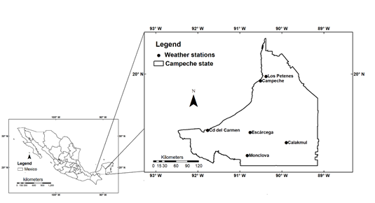
The databases for every 10 min were obtained from the automated weather stations of the National Water Commission (Comisión Nacional del Agua, Conagua) in Mexico. Table 1 shows the geographic information of the weather stations used in this study, as well as the periods of registry time from each weather station.
Table 1 Geographic information and meteorological annual conditions during the study period.
| Station | LAT (°N) | LON (°W) | ALT (msnm) | Years of registry | Annual average | |||
|---|---|---|---|---|---|---|---|---|
| Tmean (°C) | GSR MJ M-2d-1 | RH (%) | U2 (ms-1) | |||||
| Calakmul | 18.365 | 89.893 | 28 | 2000-2018 | 26.20 | 15.66 | 81.00 | 1.16 |
| Campeche | 19.836 | 90.507 | 3 | 2000-2018 | 26.80 | 20.19 | 79.90 | 1.82 |
| Cd. del Carmen | 18.658 | 91.765 | 4 | 2011-2018 | 27.10 | 19.40 | 75.16 | 2.36 |
| Escárcega | 18.608 | 90.754 | 60 | 2004-2018 | 27.17 | 18.74 | 79.2 | 1.51 |
| Los Petenes | 19.943 | 90.374 | 2 | 2012-2018 | 26.52 | 14.43 | 80.23 | 1.31 |
| Monclova | 18.057 | 90.821 | 100 | 2008-2018 | 26.70 | 18.77 | 72.59 | 1.63 |
LAT: Latitude; LON: Longitude; ALT: Altitude; Tmean: Mean temperature; GSR: Global solar radiation; RH: Relative humidity; U2 wind speed.
Management of missing data and quality
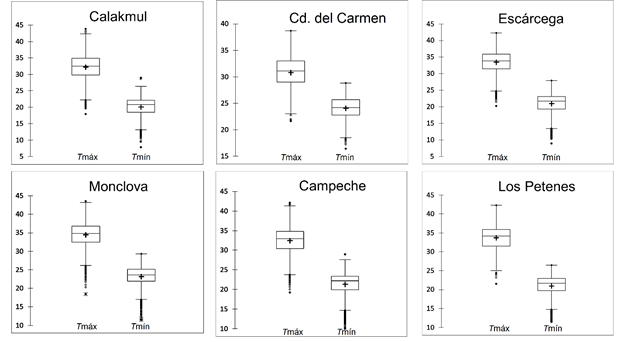
The databases were processed every 10 minutes, detecting missing series of time through algorithms implemented in the Microsoft Excel® software, which were later refilled using the interpolation technique called Piecewise Cubic Hermite Interpolating Polynomial (PCHIP). For a more detailed description, see Salazar, Ureña and Gallego (2010), and Torrente-Cantó (2018) . Once the data series were completed, daily databases were constructed. Likewise, the data were analyzed to identify atypical values, where the values above three standard deviations of the mean were marked as atypical. The data signaled as atypical were analyzed, and if an atypical extreme inferior value was associated to a rainfall event it was not eliminated; on the contrary case, it was eliminated, with the objective of having functional models even during rainy season. In the case of the atypical extreme superior values, they were eliminated; in both cases the technique of PCHIP interpolation was used to complete them. Figure 2 shows the box and whisker plots of the weather stations implied in the models of this study. The whisker represents the minimum and maximum of the variables. Concerning the maximum temperature, the mean varies between 33 and 34 °C with maximum values between 42 and 43 °C (except the station of Cd. del Carmen), the minimum value of the maximum temperature ranges between 22 and 25 °C. The minimum temperature has a mean between 20 and 24 °C, with maximum values between 25 and 28 °C and minimum between 12 and 17 °C. Figure 2 also shows the atypical values, generally associated to the minimum temperature.
FAO 56 PM (ETo-FAO56PM) equation
The FAO56PM equation is the standard model used to estimate accurately the ETo, proposed by the Food and Agriculture Organization of the United Nations (FAO). It incorporates thermodynamic and aerodynamic aspects, taking into consideration many meteorological parameters related to the process of evapotranspiration such as net radiation, air temperature, vapor pressure deficit, and wind speed. It has been shown to be a relatively accurate method under different conditions or regions (Allen et al., 1998). These aspects have been incorporated into the following equation:
where Rn = net radiation on the surface (MJ m-2 day-1); G = heat flow of the soil (MJ m-2 day-1); Tmed = mean temperature of the air at 2 m of height (°C); u2 = wind speed at 2 m of height (m s-1); es = vapor pressure at saturation (kPa); ea = real vapor pressure (kPa); ∆ = slope of the vapor pressure curve (kPa °C-1); γ = psychrometric constant (kPa °C-1).
In this study, the ETo-FAO56PM method was used to evaluate the conventional and artificial intelligence methods.
Hargreaves and Samani Equation
The HS model is considered an alternative model to estimate the ETo when only the temperature records are available in the study site; it is one of the methods that has been used consecutively because of its simple implementation and the accuracy of its results (Gong et al., 2016; Shiri, 2017). Equation (2) of the Hargreaves and Samani model is structured as follows:
where ETo = Reference evapotranspiration (mm day-1); KHG = is an empirical coefficient, which was initially established at 0.0023 but has been recalibrated according to the place used; Tmed = mean temperature; Tmax = maximum temperature; Tmin = minimum temperature; Ra = extraterrestrial solar radiation. Ra was calculated in function of the day of the year, the site’s latitude, and the solar angle according to the equation proposed by Allen et al. (1998).
Camargo equation
The Camargo model is a modification of the Thornthwaite (TH) equation; it is a model based on the climate variable of temperature. Camargo substituted the value of the mean temperature of the Thornthwaite equation by the mean effective temperature (Tef) (Camargo, Marin, Sentelhas, & Picini, 1999). Equation (3) of the Camargo model is structured in the following way:
where ETo = reference evapotranspiration (mm day-1); KCA1 and KCA2 = empirical coefficients, where their original values are 16 and 0.36, respectively, and should be calibrated according to the place of use; I = annual heat index; a= empirical exponent in function of I, N = maximum hours of sunshine; (KCA2 * (3Tmax-Tmin) = effective temperature, replacing the mean temperature in the Thornthwaite equation. The value of I is defined as the sum of 12 values of monthly heat indexes, as shown in the following equation:
where Tmedj = mean monthly temperature (°C).
and:
The value of a ranges from 0 to 4.25, while the annual heat index I varies from 0 to 160.
Parameter adjustment in conventional methods
The conventional methods based on temperature should be adjusted to the local conditions before being used (Almorox et al., 2018) to obtain good estimations of ETo; therefore, the original coefficients of the equations were calibrated by using non-linear regression techniques through the Levenberg-Marquardt algorithm.
Support Vector Machines (SVM)
The technique of support vector machines (SVM) was developed by Vapnik (2000) and is one of the approaches based on automated learning. It is a robust supervised learning technique to solve classification and regression problems applied to large sets of complex data with noise; it selects a unique hyperplane of separation of each class and the basic idea is to map the data x in a space of characteristics of high dimension through non-linear mapping and to make a linear regression in this space. During training, only the examples found in the margin of separation are considered, called support vectors. They are applied successfully in regression problems, generally called SVR (support vectors regression), using SVM for a set of data {(Xi , Yi )} N/i = 1, where Xi is the entry vector, Yi is the exit value, and N is the total number of sets of data through mapping of X in a characteristic space through a non-linear function φ(x) to later find a regression function ( Fan et al., 2018a; Mehdizadeh, Behmanesh, & Khalili, 2017; Quej, Almorox, Arnaldo, & Saito, 2017; Topi & Vanita, 2017; Wen et al., 2015):
where φ (x) is the function of non-linear mapping. ω is a weight vector and b is a bias value, they are the parameters of the regression function, which can be calculated by minimizing the following function of regularized risk:
where the term
That is, if the difference between predicted and measured values is less than ε, then the loss is equal to 0. If the predicted values are inside the tube, the loss error is equal to 0. For the rest of the predicted points found outside the tube, the loss is equal to the difference between the predicted value and the radius ε of the tube. For the detection of atypical values, the width values ξ and ξ ⃰, measure from top to bottom in the tube of ε.
Because both variables acquire positive values, the risk should be minimized with the following equation:
Subject to
where
The SVM model estimates the regression in function of a series of Kernel functions, which convert original entry data of smaller dimensions to a space of characteristics of larger size in an implicit way. Among the most used Kernels, there is polynomial SVM (SVM-Poly) and the radial base function (SVM-RBF), whose Kernel parameters ought to be adjusted previously through an algorithm. For example, the optimal Kernel parameters and the SVM model are generally obtained using the grid search method (Mehdizadeh et al., 2017):
Implementation of the SVM Model in Estimating the ETo
In this study, the SVM model to estimate the ETo was built by using the R software (RDevelopment, 2009). As entry variables, the meteorological data of Tmax, Tmin and Ra , were used, and as target variable the values of ETo-FAO56PM (Eq. 1). For training and validation of the SVM model, the R software was used together with the LIBSVM 3.1 package (Chang, Lin, & Tieleman, 2013). The Kernel Radial Base Function (RBF) was used (Eq. 10) to resize the data. With the aim of avoiding the over-adjustment and increasing the performance of the SVM model to estimate the ETo, the parameters ε, C and ɣ of the SVM, and the Kernel Radial Base Function were optimized through the genetic algorithm (GA), using cross-validation (CV= 5 folders) (Quej et al., 2017; Shrestha & Shukla, 2015), and varying the parameters ε = 0.002 to ε = 2, C = 0.0001 to C = 10, and ɣ = 0.0001 to ɣ = 2. The GA was implemented using the R software together with the e1079 and Caret library; 60 % of the data were used during the stage of training and 40 % in the stage of validation.
The parameters optimized by the GA used in the training of SVM are shown in Table 2.
Genetic Expression Programming (GEP)
Genetic expression programming (GEP) was presented by Ferreira (2001) . It is a branch of the evolutionary algorithms that has the capacity of modelling dynamic and nonlinear processes. It is an algorithm that belongs to the family of traditional genetic algorithm (GA) and genetic programming (GP). It can emulate biological evolution based on computer programming to solve a problem defined by the user.
GEPs are considered a hybrid between GA and GP. They use genetic programming for the solution of the problem in tree shape, where there are two types of nodes:
Terminal or tree leaves. They do not have descendants, and they are associated to the variables or constants.
Functions. They have descendants, and they are associated to operators of the algorithm that is attempted to be developed.
In GEP, individuals are codified first as linear chains of fixed length as in GA. Then, they are expressed as nonlinear entities of different sizes and shapes, as in GP (Ferreira, 2001). In addition, a set of terminals (coefficients and predictors), functions and mathematical operators are used in the GEP to estimate the dependent variable (Mehdizadeh et al., 2017), creating functions randomly and selecting those that present a better adjustment to the experimental results, allowing the generation of algorithms and mathematical expressions automatically for the solution of problems (Mattar, 2018; Shiri, 2017).
Implementation of the GEP model in the estimation of the ETo
In this study the implementation of the GEP technique was carried out by using the GenexprooTols V. 5.0 software, the entry variables are values of meteorological data of Tmax, Tmin, Ra and ETo-FAO56PM values as target variable. The arithmetic operators and mathematical functions implemented in the program were {
Table 3 Parameters of the GEP model.
| Parameter | Value |
|---|---|
| Number of chromosomes | 30 |
| Size of head | 8 |
| Number of genes | 3 |
| Function of link | Addition |
| Type of error in the fitness function | RMSE |
| Rate of mutation | 0.044 |
| Rate of investment | 0.1 |
| Rate of first point recombination | 0.3 |
| Rate of second point recombination | 0.3 |
| Rate of gene recombination | 0.1 |
| Rate of gene transposition | 0.1 |
| Rage of insertion sequence transposition | 0.1 |
| Root Insertion Sequence Transposition | 0.1 |
| Penalization tool | Pp* |
*Parsimony pressure.
XGBoost
It is one of the most important and potent algorithms of “Machine Learning” created by Chen and Guestrin (2016) , used for the analysis of regression problems and statistical classification, which produces a complex prediction model from the assembly of decision trees (simple models), in a context of supervised learning.
The model is based on the theory of slope increase, which is why predictions of several “weak” apprentices (models whose predictions are slightly better than random assumptions), are combined to develop a “strong” apprentice. These “weak” apprentices are combined by following a strategy of gradual learning, avoiding over-adjustment and optimizing computer resources. This is obtained by simplifying all the functions that allow combining predictive and regularization terms, but which at the same time maintain an optimal computational speed during the whole processing. At the beginning of the calibration process, a “weak” apprentice is adjusted to the entire data space, and then, a second apprentice is adjusted to the residues of the first. This adjustment process of a model to the residues of the previous one continues until some stoppage criterion is reached (minimization of the root-mean-square error). The result is a type of weighed mean of individual predictions of each weak student. Traditionally, the regression trees are selected as “weak” apprentices (Fan et al., 2018a). Under this context the XGBoost model is based in the following objective function: loss + regulator:
where l is the predictive term and Ω the regularization term. The loss function of the predictive term can be specified by the user. The regularization term is obtained as an analytical expression based on the number of tree leaves and the punctuation of each leaf. The key point of the XGBoost calibration process is that both terms are reordered in the last instance in the following expression:
where G and H are obtained from the expansion of the Taylor series of the loss function, λ is the regularization parameter, and T is the number of leaves in a tree. This analytical expression of the target function allows a fast scanning from left to right of the possible divisions of the tree, but always taking into account the complexity.
XGBoost has a broad range of adjustment parameters. In addition, the flexibility of the algorithm improves when giving the user the chance of including some auto-defined parameters, such as the loss function or the measurement used for validation and trial Urraca, Antonanzas, Antonanzas-Torres, & Martinez-De-Pison, 2017).
Implementation of the XGBoost model in the estimation of the ETo
For the implementation of the XGBoost model, as the first step, the hyper-parameters were optimized: nrounds, max_depth, eta, gamma, colsample bytree, min_child_weight, and subsample (Table 4) using the Caret library of Software R (Fan et al., 2018a); second, the XGBoost model was adjusted using the “Xgboost” library of Software R, using cross-validation (CV = 5 folders) to avoid over-adjustment. Of the data, 70 % were used for the stage of training and 30 % for validation. The entry variables to the model are the values of meteorological data of Tmax, Tmin and Ra , the ETo-FAO56PM values as target variable.
Table 4 Optimized XGBoost hyper-parameters.
| Adjusted parameters | Calakmul | Campeche | Cd. del Carmen | Escárcega | Monclova | Los Petenes |
|---|---|---|---|---|---|---|
| Nrounds | 50 | 50 | 50 | 50 | 150 | 50 |
| Max_depth | 2 | 3 | 3 | 3 | 2 | 3 |
| Eta | 0.3 | 0.3 | 0.3 | 0.3 | 0.3 | 0.3 |
| Gamma | 0 | 0 | 0 | 0 | 0 | 0 |
| Colsample bytree | 0.8 | 0.8 | 0.8 | 0.8 | 0.8 | 0.8 |
| Min_child_weight | 1 | 1 | 1 | 1 | 1 | 1 |
| subsample | 1 | 1 | 1 | 1 | 0.75 | 1 |
Statistical analysis
Four statistical indicators are used in this study to evaluate the performance of conventional and artificial intelligence models; these indicators are: coefficient of determination (R2; Eq. 13), root-mean-square error (RMSE; Eq. 14), mean absolute error (MAE; Eq. 15), mean bias error (MBE; Eq. 16):
where n is the number of comparisons, Pi and Oi are estimated and observed values of ETo-FAO56PM, respectively. Pavg is the average of estimated values of ETo, Oavg is the average of observed values of ETo. The units of ETo are shown in mm d-1.
R2 is commonly used to estimate the performance of hydrological models; it represents the fraction of estimated values that are the closest to the line of measurement data. Values of the coefficient of determination close to 1 indicate more efficient models and the regression line adjusts better to the data. The RMSE is a measurement used frequently to compare errors of prediction in different models, and the lower its value, the better the predictive capacity of a model will be in terms of its absolute deviation. MAE is the sum of absolute values of the errors divided by the number of observations, and it is used frequently to measure how close the estimated values are to the observed values. The MBE provides information about the tendency of the model to overestimate or underestimate the variable, quantifying the systematic error of the model.
The evaluation of uncertainty of statistical indicators R2, RMSE, MAE and MBE was carried out through the construction of bootstrap Intervals of Confidence (BIC) at 95 % of the level of trust, and for such a purpose the non-parametric percentile bootstrap method was used as the technique of resampling using B = 10 000 replicas with replacement with the purpose of inducing more accuracy in the estimations (Efron, 1992).
The BICs offer a way of estimating with high probability a range of values where the value of the parameter is found (statistical indicator).
The standard error of the distribution (SE) and the value of each statistical bootstrap indicator were also computed, calculating the standard deviation and the mean of the B replicas.
Results
In this study, two conventional equations were evaluated, and three artificial intelligence techniques to estimate the ETo using the air temperature variable.
Table 5 shows the statistical indexes obtained through bootstrap (mean of the bootstrap B replicas); between the conventional equations evaluated, the Camargo model showed better global results (R2 = 0.734, MAE = 0.564, RMSE = 0.721, MBE = -0.008) compared to the HS equation (R2 = 0.727, MAE = 0.588, RMSE = 0.750, MBE = -0.032), with the Monclova station presenting the best performance (R2 = 0.815; MAE = 0.488; RMSE = 0.608, MBE = -0.011). Globally, the Camargo equation had a tendency to slightly underestimate the values of ETo according to the indicator MBE = -0.008. Regarding the Camargo equation, the KCA1 coefficient ranged from 34.922 to 44.476, and the KCA2 coefficient varied from 0.195 to 0.290. In the HS equation, the calibrated KHS coefficient ranged from 0.0015 to 0.0027.
Table 5 Bootstrap statistical indexes (R2, MAE, RMSE and MBE) of the conventional and artificial intelligence models used for the estimation of the ETo from each weather station.
| Station/ model | R2 | MAE (mm d-1) | RMSE (mm d-1) | MBE (mm d-1) | KHS | KCA1 | KCA2 |
|---|---|---|---|---|---|---|---|
| Calakmul | |||||||
| HS | 0.700 | 0.569 | 0.729 | -0.055 | 0.0015 | ||
| Camargo | 0.712 | 0.534 | 0.688 | 0.028 | 36.071 | 0.200 | |
| SVM | 0.740 | 0.486 | 0.646 | 0.046 | |||
| GEP | 0.696 | 0.544 | 0.719 | -0.003 | |||
| XGBoost | 0.771 | 0.467 | 0.607 | -0.0004 | |||
| Campeche | |||||||
| HS | 0.703 | 0.550 | 0.709 | -0.010 | 0.0020 | ||
| Camargo | 0.635 | 0.623 | 0.797 | 0.037 | 40.256 | 0.218 | |
| SVM | 0.731 | 0.519 | 0.680 | -0.003 | |||
| GEP | 0.695 | 0.561 | 0.726 | 0.036 | |||
| XGBoost | 0.695 | 0.543 | 0.721 | -0.012 | |||
| Cd. del Carmen | |||||||
| HS | 0.694 | 0.633 | 0.820 | -0.002 | 0.0027 | ||
| Camargo | 0.702 | 0.627 | 0.811 | 0.005 | 44.476 | 0.240 | |
| SVM | 0.742 | 0.585 | 0.778 | -0.056 | |||
| GEP | 0.721 | 0.638 | 0.809 | -0.034 | |||
| XGBoost | 0.703 | 0.611 | 0.802 | 0.032 | |||
| Escárcega | |||||||
| HS | 0.711 | 0.654 | 0.825 | -0.050 | 0.0018 | ||
| Camargo | 0.783 | 0.554 | 0.705 | -0.036 | 38.581 | 0.211 | |
| SVM | 0.838 | 0.471 | 0.608 | 0.034 | |||
| GEP | 0.773 | 0.561 | 0.713 | 0.030 | |||
| XGBoost | 0.815 | 0.500 | 0.642 | -0.043 | |||
| Monclova | |||||||
| HS | 0.796 | 0.523 | 0.651 | 0.014 | 0.0020 | ||
| Camargo | 0.815 | 0.488 | 0.608 | -0.011 | 39.391 | 0.214 | |
| SVM | 0.852 | 0.426 | 0.531 | -0.046 | |||
| GEP | 0.816 | 0.500 | 0.618 | 0.009 | |||
| XGBoost | 0.842 | 0.442 | 0.569 | 0.025 | |||
| Los Petenes | |||||||
| HS | 0.755 | 0.599 | 0.767 | -0.089 | 0.0014 | ||
| Camargo | 0.754 | 0.555 | 0.716 | -0.071 | 34.922 | 0.195 | |
| SVM | 0.801 | 0.392 | 0.574 | -0.042 | |||
| GEP | 0.812 | 0.406 | 0.574 | -0.022 | |||
| XGBoost | 0.804 | 0.414 | 0.584 | 0.041 | |||
| All the stations | |||||||
| HS | 0.727 | 0.588 | 0.750 | -0.032 | |||
| Camargo | 0.734 | 0.564 | 0.721 | -0.008 | |||
| SVM | 0.784 | 0.480 | 0.636 | -0.011 | |||
| GEP | 0.752 | 0.535 | 0.693 | 0.003 | |||
| XGBoost | 0.772 | 0.496 | 0.654 | 0.007 | |||
* In the artificial intelligence models, the bootstrap statistical indexes correspond to those obtained in the validation process.
** KHS, KCA1, KCA2 are the empirical coefficients adjusted of the Hargreaves-Samani and Camargo equations, respectively.
Concerning the artificial intelligence models to estimate the ETo, Table 5 shows that the SVM model obtained the best performance with relation to the other models evaluated, obtaining values of R2 = 0.784, MAE = 0.480, RMSE = 0.636 and MBE = -0.011, with the Monclova station being the one that showed the best performance (R2 = 0.852; MAE = 0.426; RMSE = 0.531; MBE = -0.046); followed by the XGBoost model with results of R2 = 0.772, MAE = 0.496, RMSE = 0.654 and MBE = 0.007, where the Monclova station presented the best performance (R2 = 0.842; MAE = 0.442; RMSE = 0.569; MBE = 0.025); the GEP model was the one of lowest yield compared to the other artificial intelligence models, obtaining results of R2 = 0.752, MAE = 0.535, RMSE = 0.693 and MBE = 0.003, although their yield was higher than the one obtained by conventional equations.
The SVM model presented in general a tendency to underestimate values of ETo according to a global value of MBE=-0.011, while the GEP and XGBoost models presented a mild tendency to overestimate the values of ETo.
The SVM model has a good yield when the adjustment of the parameters of Cost, Gamma and Epsilon is done, using the Genetic Algorithm. Likewise, when using cross-validation the over-adjustment of the model is avoided.
One of the main advantages of the SVM method over the other methods lies in the non-linear problem always converging in a global minimum.
On the other hand, a useful characteristic of the GEP technique is that it provides an algebraic expression to estimate the ETo, which can be programmed in a spreadsheet, or R, Matlab or Python software. Table 6 presents the algebraic expressions obtained for the GEP model for the six weather stations.
Table 6 Algebraic expressions obtained by the GEP model for each weather station.
| Station | Mathematical expression |
|---|---|
| Calakmul |
|
| Campeche |
|
| Cd. del Carmen |
|
| Escárcega |
|
| Monclova |
|
| Los Petenes |
|
As a practical example of the GEP model, the formula is provided in the Microsoft Excel® format, whose entries correspond to the variables of Tmin, Tmax, Ra .
B2 / ((M2*Tmax) ^ (1/3)) + (ATAN(Tmax) * M3) / (ATAN(Ra -M4)) + Ra / (ATAN((Tmax-Tmin)-LOG(Ra )) +Tmin)
where M2= 0.0815; M3 = 9.223; M4 = 5.126 are constants in the model.
Thus, it is verified that when adding the values of Tmax=31.7, Tmin=18.40 and Ra = 38.87, we will obtain the value of ETo = 3.407 mm d-1.
Table 7 shows the bootstrap intervals of confidence (BIC) at 95 % level of confidence and standard error of distribution (SE) of the statistical indexes R2, MAE, RMSE and MBE of the conventional and artificial intelligence models. In general, the intervals of confidence show reduced amplitude, related to the standard error, which indicates that if we use random samples and their statistical evaluation indicators are determined, these will vary in a range that is always acceptable, as shown in Table 7.
Table 7 BIC (inferior limit [IL] = 2.5% and superior limit [SL] = 97.5%) at 95 % level of confidence and the Standard Error of distribution (SE) of the statistical indexes R2, MAE, RMSE and MBE of the conventional and artificial intelligence models.
| Station / model | R2 | MAE (mm d-1) | RMSE (mm d-1) | MBE (mm d-1) | ||||||||
|---|---|---|---|---|---|---|---|---|---|---|---|---|
| IL | SL | SE | IL | SL | SE | IL | SL | SE | IL | SL | SE | |
| Calakmul | ||||||||||||
| HS | 0.683 | 0.717 | 0.008 | 0.554 | 0.584 | 0.007 | 0.709 | 0.748 | 0.009 | -0.079 | -0.031 | 0.012 |
| Camargo | 0.696 | 0.727 | 0.007 | 0.519 | 0.548 | 0.007 | 0.669 | 0.706 | 0.009 | 0.006 | 0.049 | 0.011 |
| SVM | 0.715 | 0.765 | 0.013 | 0.462 | 0.511 | 0.012 | 0.615 | 0.677 | 0.016 | 0.009 | 0.083 | 0.019 |
| GEP | 0.667 | 0.724 | 0.014 | 0.516 | 0.572 | 0.014 | 0.682 | 0.757 | 0.019 | -0.046 | 0.039 | 0.022 |
| XGBoost | 0.757 | 0.786 | 0.007 | 0.453 | 0.482 | 0.007 | 0.589 | 0.626 | 0.009 | -0.023 | 0.023 | 0.012 |
| Campeche | ||||||||||||
| HS | 0.688 | 0.717 | 0.007 | 0.537 | 0.562 | 0.006 | 0.692 | 0.726 | 0.008 | -0.029 | 0.009 | 0.009 |
| Camargo | 0.617 | 0.652 | 0.008 | 0.609 | 0.636 | 0.007 | 0.778 | 0.815 | 0.009 | 0.014 | 0.059 | 0.011 |
| SVM | 0.707 | 0.754 | 0.011 | 0.497 | 0.54 | 0.011 | 0.652 | 0.708 | 0.014 | -0.036 | 0.029 | 0.017 |
| GEP | 0.669 | 0.72 | 0.013 | 0.537 | 0.584 | 0.012 | 0.694 | 0.758 | 0.016 | -0.001 | 0.073 | 0.018 |
| XGBoost | 0.662 | 0.727 | 0.016 | 0.517 | 0.569 | 0.013 | 0.682 | 0.759 | 0.019 | -0.052 | 0.028 | 0.021 |
| Cd. del Carmen | ||||||||||||
| HS | 0.662 | 0.726 | 0.016 | 0.603 | 0.662 | 0.015 | 0.400 | 1.241 | 0.214 | -0.049 | 0.045 | 0.024 |
| Camargo | 0.671 | 0.732 | 0.016 | 0.597 | 0.656 | 0.015 | 0.770 | 0.852 | 0.021 | -0.041 | 0.052 | 0.023 |
| SVM | 0.692 | 0.792 | 0.025 | 0.534 | 0.637 | 0.026 | 0.700 | 0.856 | 0.039 | -0.134 | 0.021 | 0.039 |
| GEP | 0.675 | 0.766 | 0.023 | 0.585 | 0.691 | 0.027 | 0.742 | 0.875 | 0.034 | -0.118 | 0.050 | 0.043 |
| XGBoost | 0.639 | 0.767 | 0.032 | 0.551 | 0.672 | 0.031 | 0.718 | 0.886 | 0.043 | -0.061 | 0.125 | 0.047 |
| Escárcega | ||||||||||||
| HS | 0.695 | 0.727 | 0.008 | 0.635 | 0.673 | 0.009 | 0.802 | 0.847 | 0.012 | -0.082 | -0.018 | 0.016 |
| Camargo | 0.769 | 0.796 | 0.007 | 0.537 | 0.570 | 0.008 | 0.685 | 0.724 | 0.010 | -0.063 | -0.009 | 0.014 |
| SVM | 0.817 | 0.859 | 0.011 | 0.445 | 0.496 | 0.013 | 0.574 | 0.642 | 0.017 | -0.006 | 0.074 | 0.021 |
| GEP | 0.745 | 0.800 | 0.014 | 0.530 | 0.592 | 0.015 | 0.677 | 0.749 | 0.018 | -0.018 | 0.079 | 0.025 |
| XGBoost | 0.791 | 0.838 | 0.012 | 0.470 | 0.531 | 0.015 | 0.606 | 0.678 | 0.018 | -0.093 | 0.006 | 0.025 |
| Monclova | ||||||||||||
| HS | 0.781 | 0.811 | 0.007 | 0.507 | 0.539 | 0.008 | 0.632 | 0.670 | 0.009 | -0.058 | -0.004 | 0.014 |
| Camargo | 0.802 | 0.829 | 0.006 | 0.473 | 0.503 | 0.007 | 0.590 | 0.626 | 0.009 | -0.036 | 0.014 | 0.013 |
| SVM | 0.832 | 0.871 | 0.009 | 0.403 | 0.449 | 0.012 | 0.503 | 0.558 | 0.014 | -0.084 | -0.007 | 0.019 |
| GEP | 0.792 | 0.839 | 0.012 | 0.471 | 0.528 | 0.014 | 0.585 | 0.651 | 0.016 | -0.037 | 0.056 | 0.024 |
| XGBoost | 0.818 | 0.866 | 0.012 | 0.412 | 0.472 | 0.015 | 0.532 | 0.605 | 0.018 | -0.022 | 0.072 | 0.024 |
| Los Petenes | ||||||||||||
| HS | 0.710 | 0.800 | 0.023 | 0.564 | 0.633 | 0.017 | 0.715 | 0.818 | 0.026 | -0.144 | -0.035 | 0.027 |
| Camargo | 0.710 | 0.798 | 0.022 | 0.523 | 0.588 | 0.016 | 0.665 | 0.767 | 0.026 | -0.122 | -0.019 | 0.026 |
| SVM | 0.724 | 0.878 | 0.039 | 0.338 | 0.446 | 0.027 | 0.463 | 0.686 | 0.057 | -0.114 | 0.030 | 0.037 |
| GEP | 0.738 | 0.886 | 0.037 | 0.352 | 0.460 | 0.027 | 0.463 | 0.684 | 0.056 | -0.097 | 0.054 | 0.038 |
| XGBoost | 0.742 | 0.866 | 0.032 | 0.353 | 0.473 | 0.030 | 0.494 | 0.674 | 0.046 | -0.042 | 0.123 | 0.042 |
Discussion
Two conventional models and three artificial intelligence techniques used to estimate values of ETo were evaluated, with the entry variables for all the models being data of Tmax, Tmin and Ra , except for the Camargo model that uses the maximum sunshine hours for a specific site, so that the models have a spatial and temporal scope of use, limited by thermal amplitude.
In the case of arid and super humid climate where there is broader thermal amplitude, Camargo et al. (1999) presented a modification to the Thornthwaite model using the term “effective temperature” Tef = 0.36 (3 Tmax - Tmin), obtaining excellent results for super humid regions in Brazil. In this study, Camargo’s empirical equation obtained better estimations of ETo in comparison to the HS equation, the latter commonly used in the Yucatan Peninsula to estimate the ETo when there are only data for temperature, this because in the stations studied there is a greater thermal amplitude. Likewise, the calibration of the KHS coefficient of the HS equation agrees with the one obtained by Bautista, Bautista and Delgado-Carranza (2009) for some sites of the Yucatan Peninsula, where the highest value of the KHS coefficient = 0.0027 was observed in the station of Cd. del Carmen surrounded by waters from the Gulf of Mexico, and the lowest values were observed in regions surrounded by abundant vegetation as in the cases of the biosphere reserves of Petenes (KHS = 0.0014) and Calakmul (KHS = 0.0015). Quej, Almorox, Arnaldo and Moratiel (2019) obtained similar results when evaluating the daily ETo using the HS and Camargo equations, obtaining values of RMSE of 0.70 and 0.80 mm d-1, respectively. Also, in a study carried out by Kelso-Bucio et al. (2013) in a regional study, the authors calibrated the empirical coefficient of the Hargreaves equation, obtained values of RMSE in the range of 0.68 to 0.87 mm d-1 for the north and central region of the state of Campeche, Mexico, values similar to this study where the RMSE value in the HS equation had a variation of 0.651 to 0.820 mm d-1.
Among the artificial intelligence techniques evaluated to estimate the ETo, the SVM model using the radial base kernel presented better results, and GEP obtained the lowest yield out of the three techniques in both stages. This agrees with the results obtained by Mehdizadeh et al. (2017) in arid and semi-arid regions of Iran where the GEP technique was implemented, two SVM models of radial base and polynomial; and MARS (Multivariate Adaptive Regression Spline) comparing it with 16 conventional equations based on mass transference, radiation and meteorological parameters; the results revealed that both MARS and SVM of radial base obtained better estimations than the rest of the artificial intelligence techniques and the conventional equations. On the other hand, the results from SVM and XGBoost techniques agree with a study carried out in China by Fan et al. (2018b), where some artificial intelligence methods were evaluated, SVM and XGBoost among them, and the results were obtained in the sub-humid climate using only air temperature data; the XGBoost technique obtained a value of RMSE = 0.723 mm d-1 and the SVM technique a value of RMSE = 0.717 mm d-1.
Finally, the XGBoost technique had a performance close to SVM. However, the use of SVM of radial base is recommended since it is a more robust technique due to its strong mathematical bases, with less computational expense by not using the data for the calculation but rather some so-called support vectors, in addition to a technique with lower tendency to over-adjust once its parameters have been adjusted via GA algorithm.
Conclusions
From the conventional equations evaluated based on temperature, the equation proposed by Camargo obtained better performance in the estimation of the ETo, which is why its use is recommended for warm sub-humid climates, as in the case of the study region. In both cases, the study provides calibrated coefficients both for stations that are located in sites close to the sea and in inland sites.
Regarding the artificial intelligence models, the SVM model of radial base is recommended to carry out estimations of the ETo.
The previous adjustment of the parameters of artificial intelligence models through algorithms is fundamental to avoid an over-adjustment that would affect future estimations using other series of data.
On the other hand, it is important to highlight that the GEP models are also a good option at the moment of performing estimations of the ETo, since the algebraic model provided by the technique could be programmed in a spreadsheet or other software, and therefore carry out predictions; and as was shown in this study, the GEP model outperformed slightly the conventional models.
The artificial intelligence models are an excellent option to estimate values of ETo since they outperform the conventional equations; however, specialized knowledge on the use of software and execution of programming codes is required for their implementation.
The models evaluated in this study can be used in regions of warm sub-humid climate and in the ranges of temperature presented in Figure 2.
In future studies the effect of relative humidity could be evaluated, as well as wind speed in the estimation of the ETo for different months of the year and under extreme conditions of rainfall.
For the implementation of the artificial intelligence models described in this study, the use of the free software R is recommended; in case of requiring codes for its implementation, they can be requested via email to this study’s author.
Acknowledgements
We thank Consejo Nacional de Ciencia y Tecnología (Conacyt) and Colegio de Postgraduados Campus Campeche for the financial support given to carry out the Master’s studies on which this research is based.
REFERENCES
Allen, R. G., Pereira, L. S., Raes, D., & Smith, M. (1998). Crop evapotranspiration. Guidelines for computing crop water requirements. FAO Irrigation and drainage paper 56. Irrigation and Drainage, 300(9), D05109. [ Links ]
Almorox, J., Senatore, A., Quej, V. H., & Mendicino, G. (2018). Worldwide assessment of the Penman-Monteith temperature approach for the estimation of monthly reference evapotranspiration. Theoretical and Applied Climatology, 131(1-2), 693-703. Recuperado de https://doi.org/10.1007/s00704-016-1996-2 [ Links ]
Antonopoulos, V. Z., & Antonopoulos, A. V. (2017). Daily reference evapotranspiration estimates by artificial neural networks technique and empirical equations using limited input climate variables. Computers and Electronics in Agriculture, 132, 86-96. Recuperado de https://doi.org/10.1016/j.compag.2016.11.011 [ Links ]
Bautista, F., Bautista, D., & Delgado-Carranza, C. (2009). Calibration of the equations of Hargreaves and Thornthwaite to estimate the potential evapotranspiration in semi-arid and subhumid tropical climates for regional applications. Atmósfera, 22(4), 331-348. [ Links ]
Čadro, S., Uzunović, M., Žurovec, J., & Žurovec, O. (2017). Validation and calibration of various reference evapotranspiration alternative methods under the climate conditions of Bosnia and Herzegovina. International Soil and Water Conservation Research, 5(4), 309-324. Recuperado de https://doi.org/10.1016/j.iswcr.2017.07.002 [ Links ]
Camargo, A. P., Marin, F. R., Sentelhas, P. C., & Picini, A. G. (1999). Adjust of the Thornthwaite’s method to estimate the potential evapotranspiration for arid and superhumid climates, based on daily temperature amplitude [JOUR]. Revista Brasileira de Agrometeorologia, 7(2), 251-257. [ Links ]
Chang, C., Lin, C., & Tieleman, T. (2013). LIBSVM : A library for support vector machines. ACM Transactions on Intelligent Systems and Technology (TIST), 307, 1-39. Recuperado de https://doi.org/10.1145/1961189.1961199 [ Links ]
Chen, T., & Guestrin, C. (2016). XGBoost: A scalable tre boosting system. KDD '16: Proceedings of the 22nd ACM SIGKDD International Conference on Knowledge Discovery and Data Mining , 19(6). Recuperado de https://doi.org/10.1145/2939672.2939785 [ Links ]
Efron, B. (1992). Bootstrap methods: Another look at the jackknife. Recuperado de https://doi.org/10.1007/978-1-4612-4380-9_41 [ Links ]
Fan, J., Wang, X., Wu, L., Zhou, H., Zhang, F., Yu, X., & Xiang, Y. (2018a). Comparison of support vector machine and extreme gradient boosting for predicting daily global solar radiation using temperature and precipitation in humid subtropical climates: A case study in China. Energy Conversion and Management, 164(January), 102-111. Recuperado de https://doi.org/10.1016/j.enconman.2018.02.087 [ Links ]
Fan, J., Yue, W., Wu, L., Zhang, F., Cai, H., Wang, X., & Xiang, Y. (2018b). Evaluation of SVM, ELM and four tree-based ensemble models for predicting daily reference evapotranspiration using limited meteorological data in different climates of China. Agricultural and Forest Meteorology, 263, 225-241. Recuperado de https://doi.org/10.1016/j.agrformet.2018.08.019 [ Links ]
Feng, Y., Cui, N., Zhao, L., Hu, X., & Gong, D. (2016). Comparison of ELM, GANN, WNN and empirical models for estimating reference evapotranspiration in humid region of Southwest China. Journal of Hydrology, 536, 376-383. Recuperado de https://doi.org/10.1016/j.jhydrol.2016.02.053 [ Links ]
Ferreira, C. (2001). Gene Expression Programming: a New Adaptive Algorithm for Solving Problems. Arxiv.org. Recuperado de https://arxiv.org/abs/cs/0102027 [ Links ]
Gong, D., Feng, Y., Jia, Y., Cui, N., Li, C., & Zhao, L. (2016). Calibration of hargreaves model for reference evapotranspiration estimation in Sichuan basin of southwest China. Agricultural Water Management, 181, 1-9. Recuperado de https://doi.org/10.1016/j.agwat.2016.11.010 [ Links ]
INEGI, Instituto Nacional de Estadística y Geografía. (2017). Anuario estadístico y geográfico de Campeche 2017. Recuperado de https://doi.org/10.1111/j.1469-8749.2009.03468.x [ Links ]
Jovic, S., Nedeljkovic, B., Golubovic, Z., & Kostic, N. (2018). Evolutionary algorithm for reference evapotranspiration analysis. Computers and Electronics in Agriculture, 150(April), 1-4. Recuperado de https://doi.org/10.1016/j.compag.2018.04.003 [ Links ]
Kelso-Bucio, H., Ba, K. M., Magaña, H. F., Sánchez, M. S., Reyes, L. D., & Pascual, R. F. (2013). Recalibración regional de los coeficientes de Hargreaves (HE y KRS) en México. XXII Congreso Nacional de Hidráulica y 1er Congreso Internacional de Ingeniería Agrícola, México. [ Links ]
Mattar, M. (2018). Using gene expression programming in monthly reference evapotranspiration modeling: A case study in Egypt. Agricultural Water Management, 198, 28-38. Recuperado de https://doi.org/S0378377417304092 [ Links ]
Mattar, M. A., & Alazba, A. A. (2019). GEP and MLR approaches for the prediction of reference evapotranspiration. Neural Computing and Applications, 31(10), 5843-5855. Recuperado de https://doi.org/10.1007/s00521-018-3410-8 [ Links ]
Mehdizadeh, S. (2018). Estimation of daily reference evapotranspiration (ETo) using artificial intelligence methods: Offering a new approach for lagged ETodata-based modeling. Journal of Hydrology, 559, 794-812. Recuperado de https://doi.org/10.1016/j.jhydrol.2018.02.060 [ Links ]
Mehdizadeh, S., Behmanesh, J., & Khalili, K. (2017). Using MARS, SVM, GEP and empirical equations for estimation of monthly mean reference evapotranspiration. Computers and Electronics in Agriculture, 139, 103-114. Recuperado de https://doi.org/10.1016/j.compag.2017.05.002 [ Links ]
Quej, V. H., Almorox, J., Arnaldo, J. A., & Moratiel, R. (2019). Evaluation of temperature-based methods for the estimation of reference evapotranspiration in the Yucatán Peninsula, Mexico. Journal of Hydrologic Engineering, 24(2). Recuperado de https://doi.org/10.1061/(ASCE) HE.1943-5584.0001747 [ Links ]
Quej, V. H., Almorox, J., Arnaldo, J. A., & Saito, L. (2017). ANFIS, SVM and ANN soft-computing techniques to estimate daily global solar radiation in a warm sub-humid environment. Journal of Atmospheric and Solar-Terrestrial Physics, 155, 62-70. Recuperado de https://doi.org/10.1016/j.jastp.2017.02.002 [ Links ]
RDevelopment, C. (2009). TEAM 2009: R: A Language and Environment for Statistical Computing. Vienna, Austria: RDevelopment. [ Links ]
Salazar, E. A. Q., Ureña, W. A., & Gallego, H. A. B. (2010). Interfaz gráfica para la interpolación de datos a través de splines. Scientia et Technica, 1(44), 195-200. [ Links ]
Shiri, J. (2017). Evaluation of FAO56-PM, empirical, semi-empirical and gene expression programming approaches for estimating daily reference evapotranspiration in hyper-arid regions of Iran. Agricultural Water Management, 188, 101-114. Recuperado de https://doi.org/10.1016/j.agwat.2017.04.009 [ Links ]
Shiri, J., Sadraddini, A. S., Nazemi, A. H., Kisi, O., Landeras, G., Fakheri Fard, A., & Marti, P. (2014). Generalizability of Gene Expression Programming-based approaches for estimating daily reference evapotranspiration in coastal stations of Iran. Journal of Hydrology, 508, 1-11. Recuperado de https://doi.org/10.1016/j.jhydrol.2013.10.034 [ Links ]
Shrestha, N. K., & Shukla, S. (2015). Support vector machine based modeling of evapotranspiration using hydro-climatic variables in a sub-tropical environment. Agricultural and Forest Meteorology, 200, 172-184. Recuperado de https://doi.org/10.1016/j.agrformet.2014.09.025 [ Links ]
Topi, P. K. P., & Vanita, N. (2017). Estimation of reference evapotranspiration using data driven techniques under limited data conditions. Modeling Earth Systems and Environment. Recuperado de https://doi.org/10.1007/s40808-017-0367-z [ Links ]
Torrente-Cantó, L. (2018). Reconstrucción basada en interpolación de Hermite aplicada a funciones discontinuas. Recuperado de http://repositorio.upct.es/handle/10317/7584 [ Links ]
Urraca, R., Antonanzas, J., Antonanzas-Torres, F., & Martinez-De-Pison, F. J. (2017). Estimation of daily global horizontal irradiation using extreme gradient boosting machines. Advances in Intelligent Systems and Computing, 527, 105-113. Recuperado de https://doi.org/10.1007/978-3-319-47364-211 [ Links ]
Vapnik, V. N. (2000). The Nature of Statistical Learning Theory (2nd ed.). New York, USA: Springer-Verlag. [ Links ]
Webb, C. P. (2010). Boreau of meteorology reference evapotranspiration calculations. (February), 20. [ Links ]
Wen, X., Si, J., He, Z., Wu, J., Shao, H., & Yu, H. (2015). Support-vector-machine-based models for modeling daily reference evapotranspiration with limited climatic data in extreme arid regions. Water Resources Management, 29(9), 3195-3209. Recuperado de https://doi.org/10.1007/s11269-015-0990-2 [ Links ]
Zhang, Z., Gong, Y., & Wang, Z. (2018). Accessible remote sensing data based reference evapotranspiration estimation modelling. Agricultural Water Management, 210(July), 59-69. Recuperado de https://doi.org/10.1016/j.agwat.2018.07.039 [ Links ]
Received: June 26, 2019; Accepted: June 28, 2020
 Este es un artículo publicado en acceso abierto bajo una licencia Creative Commons
