Genomics has evolved in recent years thanks to advances in DNA sequencing technology. This progress has allowed the generation of large amounts of data at an unprecedented speed. However, the inherent complexity of genomic data, as well as its dimensionality, pose significant obstacles¹. The diversity of genomic information, ranging from DNA sequences to associated phenotypic data, adds further complexity. In addition, variability in the quality and structure of genomic data can make it difficult to extract useful and meaningful insights. Within this context, machine learning (ML) methods emerge as valuable tools to address these challenges, offering the ability to process and analyze large volumes of data efficiently and accurately². Their ability to identify complex patterns and nonlinear relationships in genomic and phenotypic data makes them a powerful tool for knowledge extraction^2,3.

The application of ML techniques allows for addressing such tasks as the identification of genes relevant to specific traits, prediction of gene functions, detection of genetic variants associated with particular traits, and classification of species based on genomic information^4,5,6. Recently, ML has become attractive in genomic prediction because of its ability to handle large volumes of data, its flexibility in modeling nonlinear relationships, improving predictive accuracy, and continuous innovations in algorithms and techniques; nevertheless, research is needed to investigate how it compares in predicting genetic values with conventional GBLUP methods⁷. Combining genomic data with ML algorithms would lead the creation of reliable predictive and descriptive models, which in turn would have implications for selective breeding, species conservation, and the understanding of evolution^8,9.

Among the most commonly used ML methods are neural networks, support vector machines, decision trees, linear regression, and clustering methods^3,8-11. The diversity of available approaches reflects the versatility of these methods in solving challenges involving genomic information, such as DNA sequence classification and protein structure prediction¹². The success of the application of these methods in animal genomics depends to a large extent on the availability of information¹³, as well as on selecting the optimal ML method, given that several methods have been proposed, each with its own characteristics and specific predictive capabilities with different data sets and features^3,7.

Thus, the objective of this study was to compare the following ML methods -neural networks (NN), regression trees (RT), random forests (RF), and support vector machines (SVM)- to predict genomic breeding values using phenotypic records of birth, weaning and yearling weights, as well as genomic information of a population of Swiss European cattle in Mexico.

The information was drawn from the database of the Mexican Association of Registered Swiss Cattle Breeders (Asociación Mexicana de Criadores de Ganado Suizo de Registro, AMCGSR), which contains phenotypic records and animal identification, ranch of origin or owner, genealogy, and economically important traits such as birth weight (BW), weaning weight (WW) and yearling weight (YW). The data set used was previously analyzed by Valerio-Hernández et al^14,15 to fit other models, so that some of the results obtained here compare directly with those of the authors mentioned above. The treatment of phenotypic information for BW, WW, and YW followed the procedure described by Valerio-Hernández et al^14,15, i.e., individuals with missing information on maternal age, management, herd of origin, as well as individuals not genetically related were omitted. Contemporary groups (CG) were defined by combining the effects of herd, year, and time of birth. For WW, the CG were formed according to the feeding management given to the herd, as well as adjustment to specific days for weaning. CG with less than three individuals or with zero variance were discarded, according to the methodology cited above¹⁴.

Genomic information was obtained through the analysis of hair samples collected from 300 animals from ranches belonging to the AMCGSR in Colima, Jalisco, and Veracruz. Genotyping was performed by GeneSeek (Lincoln, NE, USA), using the Genomic Profile Bovine LDv.4 chip, which has been used to genotype various Bos indicus and Bos taurus breeds. A total of 150 animals were genotyped with a chip containing 30,000 markers, and another 150 animals were genotyped using a chip with 50,000 SNP (Single Nucleotide Polymorphism) markers. A total of 12,835 SNP markers present in both chips were selected.

The recoding of additive genetic effects such as AA=0, AB=1, and BB=2 and the quality control of genotypic information carried out by Valerio-Hernández et al¹⁵ were based on that performed by Jarquín et al¹⁶. For the imputation of missing genotypes in the present study, it was used the FImpute¹⁷ software (version 2.2), this process yielded 1). A marker map (marker, chromosome, base-pair position), eliminating duplicate markers or markers with unknown positions, and 2) The pedigree of the individuals and their corresponding sex. Monomorphic markers and those with a minor allele frequency (MAF) lower than 0.04 were eliminated. A total of 9,008 markers were obtained and used to build the genomic relationship matrix G; Table 1 shows the number of animals incorporated into the study for each trait after filtering.

The genomic relationship matrix G was estimated using the methodology described by Pérez-Rodríguez et al¹⁸, G=WW ^t/p, where W is the centered and standardized marker matrix and p is the total number of markers. Additionally, the relationship matrix H, which combines information from the G matrix with information from the additive genetic relationship matrix A, obtained for pedigree individuals.

Linear mixed models (Base Models). Comparison of the results of predictive power for the BW, WW, and YW breeding values considers the sequence of models and results described by Valerio-Hernández et al¹⁵ for linear mixed models versus machine learning models. In order to present all the pertinent information, the linear mixed model used by these authors is described below:

where y is the phenotype vector, X is the incidence matrix for fixed effects -which for this study are sex of the animal, age of the mother of each animal, and the contemporaneous group, described above-, b is the vector of fixed effects, Z1 is an incidence matrix connecting phenotypes with contemporaneous groups, whose effects are assumed to be random and represent the variability in phenotypes due to differences between groups of individuals that are subject to the same environmental and management conditions, c~NM(0,σgc2I), where NM denotes the multivariate normal distribution, with mean 0 and associated variance parameter σgc2, I the identity matrix, Z ₂ is an occurrence matrix connecting phenotypes with additive genetic effects which are assumed to be random effects, a∼MN(0,σa2K), with K∈{A,G,H}, e~MN(0,σe2I) represents the random error vector, where σe2 denotes the variability associated with it. Depending on the data used, model (1) gives rise to three different models, denoted as follows: 1) BLUP, K=A, 2) GBLUP, K=G, and 3) ssGBLUP (single-step GBLUP) with K=H. The linear mixed models described above were fitted by Valerio-Hernández et al¹⁵ using the BGLR statistical package¹⁹.

Machine learning models. The input variables for the ML algorithms were the genetic relationship matrix combining genomic information and pedigree information called H, as well as the effects of dam’s age for each animal, indicator variables for sex, and contemporaneous group described above. In order to include the information of the H matrix in the learning models, a spectral decomposition of the matrix was performed, i.e., H=ΓΛΓt, from which X=ΓΛ12 (main components) were obtained and utilized as covariables (explanatory variables) in the models; this and other related computational strategies have been used by other authors in the past^20,21.

Artificial neural network. Neural networks (NN) were initially designed to emulate the functioning of the nervous system and which process input information through mathematical operators, generating output values or the final result^3,22. Input variables affect model’s performance and can generate overfitting if the amount of information is large; therefore, it is important to optimize these variables²³. One of the advantages of neural networks is their ability to learn nonlinear patterns³. The model of an NN with an input layer with p predictors, a hidden layer with S neurons, and an output layer with a continuous response can be expressed as follows:

where ei~NIID(0,σe2), with NIID denoted by normal, independent, identically distributed random variables; k=1,…,S (neurons); j=1,…,p (predictors); i=1,…,n (observations), and g(⋅) represents the activation function, according to Bai et al²⁴ and Gianola et al²⁰, where, yi is the response variable for the i ^th individual, in this case, the growth weights (BW, WW, YW) of Braunvieh cattle that the network predicts as a function of inputs; β0 is the bias term or the intercept, which can represent the predicted value when the inputs are equal to zero, and wk  are weights associated with each of the neurons and determine the contribution of each neuron to the final prediction. The hidden layer is an intermediate layer between the input layer and the output layer, it is where most of the processing and feature extraction of the dataset take place; it is composed of a specific number of neurons. (S) is a hyperparameter of the model that is adjusted during the training process. A higher value of S allows the neural network to capture greater complexity in the data, but may also increase the risk of overfitting. The NN adjusts the parameters (β's, w's) during the training process to minimize the prediction error. The activation function, g(⋅), maps the real line entries to the bounded open interval (-1,1), as described by Pérez-Rodríguez et al²⁵, where gx=2/[1+exp⁡-2x]-1 is known as the hyperbolic tangent activation function (htaf). The “brnn” function was used to fit the neural network model²⁶⁾ included in the package of the same name (version 0.9.3) in the statistical package R²⁷ (version 4.3.0).

Regression trees. This model is based on the one proposed by Breiman et al²⁸, yi= ∑j=1JyjI(xiϵ Rj), where yi is a response variable (BW, WW, and YW), yj is the regression value associated with a “leaf”, xi is the set of characteristics of the observation, Rj is the region associated with “leaf j” defined by characteristics and cutoff values on the path from “root” to “leaf”. I(⋅) is an indicator function that takes the value 1 if observation i belongs to the region Rj. The tree identifies the splits that minimize the error in each region and split recursively until a process-stopping criterion is reached, such as the maximum depth of the tree or the minimum number of cases in a leaf. The model fitting was performed with the “rpart” function²⁹⁾ included in the library of functions of the same name (version 4.1.19) within the statistical package²⁷ (version 4.3.0).

Random forests. This model combines multiple RTs averaging the predictions of each to obtain a final optimized prediction, yi= 1N∑j=1Nyij, where N is the number of trees in the random forest, yi is an observed random variable (BW, WW, and YW), and yij is the prediction of the j ^th RF for the observation i. The random forests algorithm was implemented using the “randomForest” function³⁰ included in the library of functions of the same name (version 4.7-1.1) within the statistical package R²⁷ (version 4.3.0).

Support vector machine. The Support Vector Machine Model (SVM) was used for classification and regression³¹. Within the context of regression, given a data set y1,x1,…,{yn,xn}, where yi represents the value of the continuous response variable for the i ^th individual, and xi, the value of the associated covariates, the objective is to obtain a function f(x) such that the distance with y is no larger than ε for each of the training points. According to Hastie et al.³² the regression function is approximated in terms of basis functions hmx,m=1,…,M as follows:

where β=(β0,β1,…,βM)t are coefficients obtained by minimizing: Qβ=∑i=1nLyi-fxi+λ2∑βm2, in which L(⋅) is called loss function (e.g. quadratic or absolute value), and λ is a positive regularization parameter. For any selection of L(⋅), the solution has the form: f^x=∑i=1na^iK(x,xi), with K(⋅,⋅) known as kernel function. Kernels are fundamental components of the model; they serve as functions that allow transforming the data and generating a higher dimensional space; they help to model complex relationships in the data. The most common kernels are the linear (xitxj), polynomial (xitxj+coef0)d,d=2,3,…, radial e-γxi-xj2, and sigmoid (htaf⁡(γxitxj), +coef0), where γ is known as the bandwidth that is adjusted in the training process through cross-validation, and coef0 is a constant that can be adjusted during the model training process, although it is usually set to 1. The model was fitted using the “e1071” package³³ (version 1.7-13), with the help of the SVM function in the statistical package R²⁷ (version 4.3.0). Codes for model fitting are available upon request to the author for correspondence.

Cross-validation. Cross-validation is a widely used data re-sampling method to estimate the true prediction error of models and to adjust model parameters^20,34. Therefore, in order to obtain the predictive capability of the models NN, RT, RF, and SVM, and thus make the comparison, the cross-validation was carried out using as a reference the procedures performed by Valerio-Hernández et al¹⁵ These authors randomly divided the data into percentages, allotting 80 % to the training set and 20 % to the validation set, and the process was repeated 100 times. The ML models were fitted, and the correlations between the observed vs. predicted values were estimated by observing the values of the response variable corrected for fixed effects and other random effects. Pearson's correlation coefficient was estimated for the corrected phenotypes and predicted genetic values for each one of the partitions, and averages were obtained for each model.

Table 2 presents the averages of the 100 Pearson correlations (based on cross-validation) between corrected and predicted values for the BW, WW, and YW traits, using the four ML algorithms compared in the study. For WW, the SVM algorithm achieved the highest values for the Pearson’s correlation coefficient between corrected and predicted values in the validation sets (WW= 0.256). By this method, the best fit for the three characteristics was obtained with the “Radial Kernel” by optimizing the hyperparameters γ (gamma) and cost (BW: 0.045 and 0.05; WW and YW: 0.05 and 0.01, respectively). Tests performed using the Artificial NN method determined the number of neurons in the hidden layer of the model to be 3 neurons for BW and 2 for WW and YW when appropriate parameter estimators of weights were obtained generating a parsimonious model. The best performance of this method was estimated at 0.402 for the BW and 0.195 for the YW.

For the RF method, tests were conducted with different numbers of “trees” as model parameters; 150 of these obtained optimal prediction values for BW and WW, and 250, for YW. The third-best performance values were predicted for WW and YW. The RT methodology showed lower predictive capacity for WW and YW in this study. Based on these results, the following set of hypotheses were proposed to test the significance of the estimated correlation coefficients: H0:μr≤0vsH1:μr>0, where μr is the mean of the distribution of the Pearson correlation coefficient and it was to test whether the association is positive or not. The set of hypotheses was tested using the 1-sample t-test, first verifying the assumption of normality in each of the cases³⁵; in all cases, it was concluded that the assumption of normality is appropriate (P-value>0.05).

To determine the predictive ability of the ML models, Pearson correlation coefficient estimators between corrected phenotypes and predicted genetic values were compared with those obtained from the analyzed models³⁶ in the test sets for each characteristic of the cross-validation methodology described above; unlike the previous studies, this study maintained consistency in the data used in the analyses. This ensures consistency in the comparisons made and provides a solid basis for evaluating the relative performance of traditional methods and ML algorithms. The problem of inferring genetic values and predicting phenotypes for quantitative traits governed by complex forms of gene interactions is difficult to solve using the routinely used linear mixed models^37,38, Therefore, the use of ML algorithms is an alternative to model complex functions by identifying nonlinear relationships between the covariates and the response variable²⁰. The correlations between corrected phenotypes and predicted values with the methodologies used made it possible to evaluate the NN, RT, RF, and SVM machine learning algorithms for the growth characteristics BW, WW, and YW in bovines. Figure 1 illustrates that the NN, RF, and SVM algorithms generally showed a similar predictive performance to that of the methodologies assessed by Valerio-Hernandez et al¹⁵ using the same variables. In a study comparing the predictive capacity of nonlinear neural networks (NLNN) with linear models, these were found to be potentially useful to predict complex characteristics based on genomic information, a situation in which the number of parameters to be estimated usually exceeds the sample size²⁰. Rodríguez-Alcántar³ compared ML algorithms using different sets of SNPs generated from chromosomes with a high number of QTLs associated with high milk production. This author found that classification accuracy ranged between 90.9 and 94.5 % with decision trees, and between 79.0 and 87.3 % with neural networks. The author concludes that both the neural network method for binary classification and decision trees are efficient tools for the early identification of highly producing dairy cows.

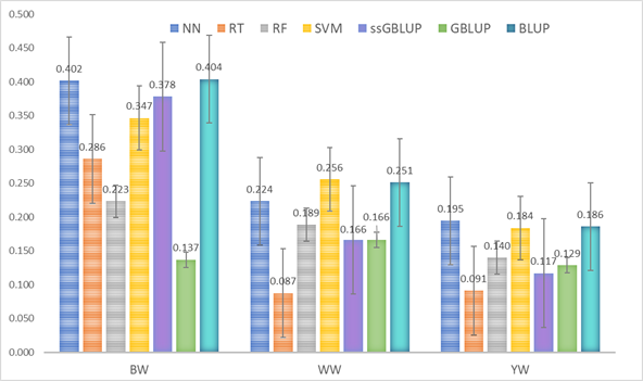
Genetic values obtained with machine learning methods, artificial neural networks (NN), regression trees (RT), random forests (RF), and support vector machines (SVM) with the methodologies applied by Valerio-Hernández et al¹⁵, best linear unbiased predictor (BLUP), genomic BLUP (GBLUP) and single-step GBLUP (ssGBLUP) for birth weight (BW), weaning weight (WW) and yearling weight (YW) of a population of Braunvieh cattle.

Figure 1 Comparison of correlation coefficients (average of 100 validations) of corrected phenotypes and predicted genetic values 

The results suggest that the performance of the models varies according to the feature and the amount of information²⁰, among other factors. This suggests that better results can be obtained with these models by including more variable and covariate information to fit the training model^39,40; despite the low correlations and large variances of the predictions, these can be attributed to several genetic and methodological factors. Consistently with the findings of Cuyabano et al⁴¹, it is important to consider genetic differences between reference and target populations when calculating the accuracy of predictions. Furthermore, it is suggested that there is a theoretical upper limit to the accuracy of these predictions, determined by the square root of the heritability. Zhang et al⁴² mention that various factors can influence the accuracy of genomic breeding value predictions; heritability (using the model described as BLUP, Valerio-Hernandez et al¹⁵ report 0.260 for BW; 0.223 for WW, and 0.231 for YW), the density of genetic markers, the minor allele frequency (MAF) utilized during the data cleaning process, and the statistical model used are just some factors that can affect the accuracy of genomic breeding value predictions. This poses significant challenges in the prediction of complex traits.

The SVM, NN, and RF methodologies showed similar performance in terms of Pearson correlation coefficients of corrected phenotypes and predicted values for the three growth characteristics used; these results were subsequently compared with the values obtained by Valerio-Hernández et al¹⁵ using traditional BLUP, GBLUP, and ssGBLUP methodologies. The computational cost of the BW was higher than that of the other three compared algorithms; it was determined by measuring the runtime required to train and validate each one of the algorithms on this training and test data sets, recording the time elapsed from the start of the training to the completion of the validation process. This result is similar to that reported by Zhao et al⁴³, who mentioned that NR adjustment is more complicated and time-consuming. The SVM algorithm stood out as a promising tool for prediction based on genomic information, considering the amount of information and the parameters used with this methodology. Like the Kernel³¹, this algorithm contributes to ML applications for the analysis of datasets derived from genetic and genomic information^44,45.

The results obtained in this study prove that ML algorithms have the potential to generate useful predictions even under constrained information conditions, such as a small sample size and low density of genetic markers. This finding highlights their applicability in practical scenarios where resources are limited. Nevertheless, significant challenges were identified, such as high computational cost and dependence on sufficient quality data to maximize predictive capability. Despite these limitations, algorithms such as NN and SVM showed consistent performance, suggesting that they may be valuable tools for genomic analysis. These results not only provide practical insights on the use of ML algorithms, but also open the door to future research focused on evaluating their behavior with larger and more detailed databases, optimizing both their implementation and their predictive capacity within different contexts.

REFERENCES

1. Pérez-Enciso M, Steibel JP. Phenomes: the current frontier in animal breeding. Genet Sel Evol 2021;53(1):22. doi: 10.1186/s12711-021-00618-1. PMID: 33673800; PMCID: PMC7934239. [ Links ]
2. Song H, Dong T, Yan X, Wang W, Tian Z, Hu H. Using Bayesian threshold model and machine learning method to improve the accuracy of genomic prediction for ordered categorical traits in fish. Agric Comm 2023;1(1):100005. https://doi.org/10.1016/j.agrcom.2023.100005. [ Links ]
3. Rodríguez-Alcántar E. Aplicación de algoritmos de aprendizaje automático para la clasificación de ganado lechero utilizando SNP de genoma completo [tesis Doctorado]. Baja California, México: Universidad Autónoma de Baja California; 2019. [ Links ]
4. Campos TL, Korhonen PK, Hofmann A, Gasser RB, Young ND. Harnessing model organism genomics to underpin the machine learning-based prediction of essential genes in eukaryotes - Biotechnological implications. Biotechnol Adv 2022;54:107822. https://doi.org/10.1016/J.BIOTECHADV.2021.107822. [ Links ]
5. Zhao T, Wu H, Wang X, Zhao Y, Wang L, Pan J, et al. Integration of eQTL and machine learning to dissect causal genes with pleiotropic effects in genetic regulation networks of seed cotton yield. Cell Rep 2023;42(9). https://doi.org/10.1016/j.celrep.2023.113111. [ Links ]
6. Guo T, Li X. Machine learning for predicting phenotype from genotype and environment. Curr Opin Biotechnol 2023;79:102853. https://doi.org/10.1016/J.COPBIO.2022.102853. [ Links ]
7. Wang X, Shi S, Wang G, Luo W, Wei X, Qiu A, et al. Using machine learning to improve the accuracy of genomic prediction of reproduction traits in pigs. J Anim Sci Biotechnol 2022;13(60). https://doi.org/10.1186/s40104-022-00708-0. [ Links ]
8. Long N, Gianola D, Rosa GJM, Weigel KA. Application of support vector regression to genome-assisted prediction of quantitative traits. Theor Appl Genet 2011;123(7):1065-1074. https://doi.org/10.1007/s00122-011-1648-y. [ Links ]
9. González‐Camacho JM, Ornella L, Pérez‐Rodríguez P, Gianola D, Dreisigacker S, Crossa J. Applications of machine learning methods to genomic selection in breeding wheat for rust resistance. Plant Genome 2018;11(2):170104. https://doi.org/10.3835/plantgenome2017.11.0104. [ Links ]
10. Müller AC, Guido S. Introduction to Machine Learning with Python: A guide for data scientists. O'Reilly Media, Inc. 2016. [ Links ]
11. Azodi CB, Bolger, E, McCarren, A, Roantree, M, de los Campos, G, Shiu, SH. Benchmarking parametric and machine learning models for genomic prediction of complex traits. G3: Genes, Genomes, Genetics 2019;9(11):3691-3702. https://doi.org/10.1534/g3.119.400498. [ Links ]
12. Fa R, Cozzetto D, Wan C, Jones DT. Predicting human protein function with multitask deep neural networks. PLoS ONE 2018;13(6). https://doi.org/10.1371/journal.pone.0198216. [ Links ]
13. VanRaden PM. Efficient methods to compute genomic predictions. J Dairy Sci 2008;91(11):4414-4423. https://doi.org/10.3168/jds.2007-0980. [ Links ]
14. Valerio-Hernández JE, Pérez-Rodríguez P, Ruíz-Flores A. Quantile regression for prediction of complex traits in Braunvieh cattle using SNP markers and pedigree. Rev Mex Cienc Pecu 2023;14(1):172-189. https://doi.org/10.22319/rmcp.v14i1.6182. [ Links ]
15. Valerio-Hernández JE, Ruíz-Flores A, Nilforooshan MA, Pérez-Rodríguez P. Single-step genomic evaluation for growth traits in a Mexican Braunvieh cattle population. Anim Biosci 2023;36(7):1003-1009. https://doi.org/10.5713/ab.22.0158. [ Links ]
16. Jarquín D, Howard R, Graef G, Lorenz A. Response surface analysis of genomic prediction accuracy values using quality control covariates in soybean. Evol Bioinform Online 2019;15:1176934319831307. https://doi.org/10.1177/117693431 9831307. [ Links ]
17. Sargolzaei M, Chesnais JP, Schenkel FS. A new approach for efficient genotype imputation using information from relatives. BMC Genomics 2014;15:478. https://doi.org/10.1186/1471-2164-15-478. [ Links ]
18. Pérez-Rodríguez P, Crossa J, Rutkoski J, Poland J, Singh R, Legarra A, et al. Single-step genomic and Pedigree Genotype × Environment interaction models for predicting wheat lines in international environments. Plant Genome 2017;10(2). https://doi.org/10.3835/plantgenome2016.09.0089. [ Links ]
19. Pérez P, de los Campos G. Genome-wide regression and prediction with the BGLR statistical package. Genetics 2014;198:483-95. https://doi.org/10.1534/genetics.114.164442. [ Links ]
20. Gianola D, Okut H, Weigel KA, Rosa GJM. Predicting complex quantitative traits with Bayesian neural networks: a case study with Jersey cows and wheat. BMC Genetics 2011;12:87. doi.org/10.1186/1471-2156-12-87. [ Links ]
21. Pérez-Rodríguez P, Flores-Galarza S, Vaquera-Huerta H, del Valle-Paniagua DH, Montesinos-López OA, Crossa J. Genome-based prediction of Bayesian linear and non-linear regression models for ordinal data. Plant Genome 2020;13(2). https://doi.org/10.1002/tpg2.20021. [ Links ]
22. Peng J, Yan G, Druzhinin Z. Applying an artificial neural network- Developed collective animal behavior algorithm for seismic reliability evaluation of structure. Measurement 2023;220:113355. [ Links ]
23. Wang C, Xu S, Liu J, Yang J, Liu C. Building an improved artificial neural network model based on deeply optimizing the input variables to enhance rutting prediction. Constr Build Mater 2022;348:128658. [ Links ]
24. Bai S, Kolter JZ, Koltun V. An empirical evaluation of generic convolutional and recurrent networks for sequence modeling. CoRR 2018. http://arxiv.org/abs/1803.01271. [ Links ]
25. Pérez-Rodríguez P, Gianola D, Weigel KA, Rosa GJM, Crossa J. An R package for fitting Bayesian regularized neural networks with applications in animal breeding. J Anim Sci 2013;91(8):3522-3531. https://doi.org/10.2527/jas.2012-6162. [ Links ]
26. Pérez-Rodriguez P, Gianola D. Title Bayesian regularization for Feed-Forward Neural Networks. 2022. https://cran.r-project.org/package=brnn. [ Links ]
27. R Core Team. R: A language and environment for statistical computing. R Foundation for statistical computing. 2021. Vienna, Austria. https://www.R-project.org/. [ Links ]
28. Breiman L, Friedman JH, Olshen RA, Stone CJ. Classification and Regression Trees. Wadsworth. 1984. https://doi.org/10.1201/9781315139470. [ Links ]
29. Therneau T, Atkinson B, Ripley B. Package “rpart”. 2022. https://cran.r-project.org/package=rpart. [ Links ]
30. Liaw A, Wiener M. Classification and Regression by random Forest. R News 2002;2(3): 18-22. https://CRAN.R-project.org/doc/Rnews/. [ Links ]
31. Chih-Chung C, Chih-Jen L. LIBSVM: A library for support vector machines. ACM Trans Intell Syst Technol 2011;2(3):1-27. http://www.csie.ntu.edu.tw/~cjlin/libsvm. [ Links ]
32. Hastie T, Tibshirani R, Friedman J. The elements of statistical learning: Data mining, inference, and prediction. Berlin: Springer Science & Business Media. 2008. [ Links ]
33. Meyer D, Dimitriadou E, Hornik K, Weingessel A, Leisch F, Chang C, Lin C. Package “e1071”. 2023. https://cran.r-project.org/package=e1071. [ Links ]
34. Berrar D. Cross-Validation. ABC of bioinformatics. Elsevier 2018; 542-545. https://doi.org/10.1016/B978-0-12-809633-8.20349-X. [ Links ]
35. Royston P. An extension of Shapiro and Wilk's W test for normality to large samples. Applied Statistics 1982;(31):115-124. https://doi.org/10.2307/2347973. [ Links ]
36. González-Recio O, Forni S. Genome-wide prediction of discrete traits using bayesian regressions and machine learning. Genet Sel 2011;43(1): https://doi.org/10.1186/1297-9686-43-7. [ Links ]
37. Gianola D, de los Campos G. Inferring genetic values for quantitative traits non-parametrically. Genet Res (Camb) [Internet]. 2009/01/06. 2008;90(6):525-540. [ Links ]
38. Gianola D, Fernando RL, Stella A. Genomic-Assisted prediction of genetic value with semiparametric procedures. Genetics 2006;173(3):1761-1776. https://doi.org/10.1534/genetics.105.049510. [ Links ]
39. Monaco A, Pantaleo E, Amoroso N, Lacalamita A, Lo Giudice C, Fonzino A, et al. A primer on machine learning techniques for genomic applications. Comput Struct Biotechnol J 2021;19:4345-4359. https://doi.org/10.1016/j.csbj.2021.07.021. [ Links ]
40. Alves AAC, da Costa RM, Bresolin T, Fernandes Júnior GA, Espigolan R, Ribeiro AMF, et al. Genome-wide prediction for complex traits under the presence of dominance effects in simulated populations using GBLUP and machine learning methods. J Anim Sci 2020;98(6):1-11. https://doi.org/10.1093/jas/skaa179. [ Links ]
41. Cuyabano BCD, Boichard D, Gondro C. Expected values for the accuracy of predicted breeding values accounting for genetic differences between reference and target populations. Genet Sel Evol 2024;56:15. https://doi.org/10.1186/s12711-024-00876-9. [ Links ]
42. Zhang H, Yin L, Wang M, Yuan X, Liu X. Factors affecting the accuracy of genomic selection for agricultural economic traits in maize, cattle, and pig populations. Front Genet 2019;14(10):189. https://doi.org/10.3389/fgene.2019.00189. [ Links ]
43. Zhao W, Lai X, Liu D, Zhang Z, Ma P, Wang Q, et al. Applications of support vector machine in genomic prediction in pig and maize populations. Front Genet 2020;11:598318. https://doi.org/10.3389/fgene.2020.598318. [ Links ]
44. González-Camacho JM, Ornella L, Pérez-Rodríguez P, Gianola D, Dreisigacker S, Crossa J. Applications of machine learning methods to genomic selection in breeding wheat for rust resistance. Plant Genome 2018;11(2). https://doi.org/10.3835/plantgenome2017.11.0104. [ Links ]
45. Libbrecht M, Noble W. Machine learning applications in genetics and genomics. Nat Rev Genet 2015;16:321-332. https://doi.org/10.1038/nrg3920. [ Links ]
Received: January 08, 2024; Accepted: November 28, 2024
Este es un artículo publicado en acceso abierto bajo una licencia Creative Commons