


 nueva página del texto (beta)
 Inglés (pdf)
 Artículo en XML
 Referencias del artículo
 Enviar artículo por email
 Citado por SciELO
  Similares en
SciELO
Similares en
SciELO 
 Permalink
Introduction
Biodiversity knowledge requires a good inventory of taxa in the region of interest. Mexico has the fifth richest flora in the world with more than 24,000 species (Sosa et al., 2023; Ulloa-Ulloa et al., 2017; Villaseñor, 2016; Villaseñor & Meave, 2022), which is distributed throughout a wide range of habitats. This richness results from the country’s heterogeneous geography, which causes a varied topography and climatic regimes.
Regional diagnoses put floristic knowledge into perspective and can be informative as strategies to improve biodiversity knowledge at that scale. To date, such diagnoses have been performed for northern Mexico (González-Elizondo et al., 2017) and the Yucatán Peninsula (Pérez-Sarabia et al., 2017). On the other hand, the National Commission for the Knowledge and Use of Biodiversity (Conabio) has coordinated a series of publications entitled State Studies, which contain a diagnosis of biodiversity, including plants, for each state. By 2022, the official Conabio website reported the publication of 24 state studies, which provides an idea of the magnitude of plant diversity in each of the evaluated states (https://www.biodiversidad.gob.mx/region/EEB/estudios). However, 60% of these studies unfortunately do not include a floristic inventory, which limits their usefulness for the specific characterization and comparison of flora across states.
Mexico’s floristic knowledge, although still fragmented, is approaching a level that allows the identification of diversity patterns that would have been impossible to achieve 2 or 3 decades ago. At present, in addition to the biodiversity information discussed in the state studies, floristic inventories have been published for 24 of the 32 Mexican states. This has increased from the 18 state inventories counted by Villaseñor (2016), adding Sinaloa (Vega-Aviña et al., 2021), Hidalgo (Villaseñor et al., 2022), Coahuila, Nuevo León, and Tamaulipas (Villaseñor et al., 2023). Furthermore, regional and local inventories provide additional information that helps to synthesize the floristic richness of each state where they were carried out (Villaseñor & Meave, 2022).
Inventories at the state level help to understand floristic diversity in various ways, for example, to comprehend the taxonomic composition, the environments within the state where species are distributed, the levels of endemism (at both the national and state levels) or restrictedness (non-endemic known from a single state), etc. In addition, the decisions on the conservation of biodiversity are carried out alternately between the federal and state governments (Íñiguez-Dávalos et al., 2015). Hence, a good knowledge of a state’s flora is essential for the success of conservation strategies.
In this study, we used a database of the floristic knowledge of the Mexican flora at the state level to examine patterns of floristic similarities. The database included the occurrence by state of all vascular plants recognized as constituting the flora of Mexico. Species were grouped by state occurrence to generate maps of total diversity and the richness documented in each main biome. We focused on determining variations in floristic composition among the 32 Mexican states.
This paper postulates that floristic composition in the Mexican states follows a geographical association and that states that are geographically close to each other will show assemblages that are defined by their floristic elements (species). In addition, these assemblages (floristic units or regions) are related to the biomes found in their territory in response to the abiotic features (climate, soil, topography, etc.) that characterize each biome. We used a descriptive approach to note floristic similarities between states, as a classification exercise to understand species’ distributions.
Materials and methods
We compiled a database containing the list of known species for each Mexican state (Operational Geographic Unit or OGU), which was an update of the information reported in recent inventories (Villaseñor, 2016; Villaseñor & Meave, 2022) and summarized in Abamap (Serrano-Estrada et al., 2022, https://abamap2.abaco2.org/). It included the species richness for each state. For each species, we also included the biome(s) (Villaseñor & Ortiz, 2014) where it has been recorded, based on literature review or specimens housed in different herbaria in Mexico and abroad, provided as online resources (Conabio, http://www.conabio.gob.mx; IBdata, https://www.ibdatav4pgsql.virtualhalls.net/web/; TROPICOS, http://www.tropicos.org).
We used the records to build an incidence matrix to evaluate floristic similarities. Using the states as OGUs, we carried out a floristic similarity analysis utilizing the Sørensen-Dice similarity coefficient and WPGMA as the grouping method. The Sørensen-Dice coefficient is among the most used and recommended to analyze presence-absence data (e.g., Vellend, 2001), and WPGMA is the preferred clustering method, since it weights the contributions of the groupings considering the number of terminal nodes (states) they contain, ensuring that each contributes equally to each nesting to which it belongs (González-Orozco et al., 2014). The analyses were carried out using NTSYS-pc software, version 2.21 (Rohlf, 2007). The floristic similarities among the states and the biomes were explored and mapped. On one hand, this allowed us to evaluate floristic relationships among the states and to identify potential floristic regions (assemblages or floristic units); but, most importantly, it allowed us to identify the main floristic elements (species) that characterize each chorology (floristic unit).
We used information on the species’ occurrence by biome to evaluate floristic similarities among the states according to the number of species recorded in each of the 5 major biomes in Mexico (Villaseñor & Ortiz, 2014). For this analysis, we included only the species occurring in 3 or fewer biomes; those recorded in 4 or 5 biomes were discarded. This selection was intended to evaluate just those species characterizing the biome and at least 2 contiguous biomes. All these floristic assessments were compared to evaluate possible similarities between the floristic groups obtained based on total richness and those based on the subset of species occurring in the different biomes found in the state.
Results
A total of 23,412 native species were documented and analyzed (Supplementary material). This figure does not include 1,118 species recorded as exotic (introduced) and naturalized; although they are part of the country’s floristic diversity, this study focused on native species. The greatest number of species occurred in the states located in southeastern Mexico: Oaxaca (10,534), Chiapas (9,313), and Veracruz (8,992, Table 1). The median number of species per state is 4,335.5, ranging from a minimum of 1,479, recorded in Tlaxcala, to a maximum of 10,534, recorded in Oaxaca.
Table 1 Floristic richness recorded in the Mexican states overall and in each of the major biomes. V2016 = Species according to Villaseñor (2016), Species = figures reported in this study, HMF = Humid Mountain Forest, HTF = Humid Tropical Forest, STF = Seasonally Dry Tropical Forest, TEM = Temperate Forest, XER = Xerophytic Scrub. The full names of the states are indicated in Figure 1. An asterisk indicates the absence of the biome in the state.
| State | V2016 | Species | HMF | HTF | STF | TEM | XER |
|---|---|---|---|---|---|---|---|
| AGS | 1,871 | 2,251 | 367* | 64* | 553 | 1,068 | 930 |
| BC | 2,336 | 2,408 | 64* | 49* | 453 | 543 | 1,542 |
| BCS | 1,988 | 2,108 | 92* | 106* | 735 | 440 | 1,256 |
| CAMP | 2,369 | 2,472 | 495* | 1,275 | 787 | 299 | 210* |
| CHIS | 8,790 | 9,313 | 3,781 | 4,047 | 2,064 | 2,621 | 751* |
| CHIH | 4,291 | 5,055 | 625* | 227* | 1,239 | 2,403 | 2,317 |
| CDMX | 1,978 | 1,979 | 549 | 69* | 332* | 1,032 | 633 |
| COAH | 3,780 | 4,097 | 456* | 134* | 596 | 1,795 | 2,444 |
| COL | 4,333 | 2,812 | 652 | 574 | 1,073 | 767 | 323 |
| DGO | 4,472 | 5,701 | 956 | 457* | 1,578 | 2,761 | 2,094 |
| GTO | 3,206 | 3,551 | 714* | 171* | 828 | 1,633 | 1,393 |
| GRO | 6,551 | 7,120 | 2,279 | 1,551 | 2,548 | 2,901 | 1,090 |
| HGO | 4,734 | 5,195 | 1,706 | 752 | 1,015 | 2,312 | 1,632 |
| JAL | 7,155 | 7,608 | 1,983 | 1,257 | 2,621 | 3,400 | 1,530 |
| MEX | 5,177 | 5,557 | 1,524 | 671 | 1,681 | 2,612 | 1,223 |
| MICH | 5,885 | 6,458 | 1,768 | 1,054 | 2,364 | 2,734 | 1,209 |
| MOR | 3,491 | 3,848 | 975 | 464* | 1,228 | 1,560 | 793 |
| NAY | 3,964 | 4,391 | 1,034 | 835 | 1,591 | 1,680 | 689 |
| NL | 3,740 | 4,161 | 604 | 179* | 613 | 1,855 | 2,110 |
| OAX | 10,229 | 10,534 | 3,889 | 3,352 | 2,964 | 3,934 | 1,727 |
| PUE | 5,232 | 6,638 | 2,180 | 1,416 | 1,782 | 2,659 | 1,710 |
| QRO | 4,411 | 4,609 | 1,252 | 567* | 1,006 | 1,943 | 1,593 |
| QROO | 2,276 | 2,393 | 465* | 1,235 | 747 | 264* | 183* |
| SLP | 5,413 | 5,673 | 1,390 | 856 | 1,243 | 2,286 | 2,154 |
| SIN | 3,736 | 4,280 | 844 | 575 | 1,689 | 1,671 | 950 |
| SON | 4,106 | 4,661 | 508* | 266* | 1,364 | 1,932 | 2,136 |
| TAB | 2,826 | 3,641 | 1,105 | 2,194 | 778* | 551* | 164* |
| TAMS | 4,278 | 5,107 | 1,041 | 706 | 1,034 | 1,953 | 1,983 |
| TLAX | 1,297 | 1,479 | 403* | 42* | 214 | 781 | 495 |
| VER | 8,497 | 8,992 | 3,339 | 3,362 | 1,914 | 3,020 | 1,584 |
| YUC | 1,900 | 2,042 | 322* | 953 | 727 | 217* | 219 |
| ZAC | 3,705 | 3,894 | 660* | 206* | 1,007 | 1,890 | 1,552 |
| Total | 23,314 | 23,412 | 5,922 | 5,031 | 5,414 | 8,912 | 6,008 |
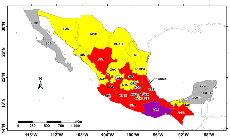
Figure 1 Species richness by state represented by quartiles (see Table 1 for raw values). Gray = first quartile (Q1 = 2,726.5 species), yellow = second quartile (Q2 = 4,335.5), red = third quartile (Q3 = 5,680 species), and purple = fourth quartile (Q4 = 10,534 species). AGS = Aguascalientes, BC = Baja California, BCS = Baja California Sur, CAMP = Campeche, COAH = Coahuila, COL = Colima, CHIS = Chiapas, CHIH = Chihuahua, CDMX = Mexico City, DGO = Durango, GTO = Guanajuato, GRO = Guerrero, HGO = Hidalgo, JAL = Jalisco, MEX = Estado de México, MICH = Michoacán, MOR = Morelos, NAY = Nayarit, NL = Nuevo León, OAX = Oaxaca, PUE = Puebla, QRO = Querétaro, QROO = Quintana Roo, SLP = San Luis Potosí, SIN = Sinaloa, SON = Sonora, TAB = Tabasco, TAMPS = Tamaulipas, TLAX = Tlaxcala, VER = Veracruz, YUC = Yucatán, ZAC = Zacatecas. Map by E. Ortiz.
Figure 1 shows the quartile of species richness for each state. The states located on both peninsulas (Baja California and Yucatán) had lower species richness than the more continental states. The 4 states with the smallest area (Aguascalientes, Colima, Mexico City, and Tlaxcala) had comparatively low richness. Morelos, which is similar in area to these states, had greater species richness, placing it in the second quartile. The states located in the north of the country, except Durango, had lower richness than those in the south, with Oaxaca standing out as the state with the greatest plant richness.
Richness by biome. Table 1 shows the number of species in each state by biome. The 14,915 species that are documented as present in 3 or fewer biomes, which were considered for analyses by biome, accounted for 63.7% of the total richness. Not all biomes occur in each state (Table 1). However, we classified for the biome any species recorded in another state where it positively occurs. For example, in Baja California there are no Humid Mountain Forests (HMF) or Humid Tropical Forests (HTF), but 64 species recorded in the state are distributed in HMF and 49 in HTF in other states. In Tabasco, Xerophytic Scrub (XER) is not documented, but 164 species that are characteristic of the XER are documented in its flora, mainly associated with coastal communities.
The greatest richness of species by biome did not always follow the same pattern as the total richness. When considering richness by biome, the 3 richest states for each biome were as follows: for Humid Mountain Forest (HMF) Oaxaca, Chiapas, and Veracruz; for Humid Tropical Forest (HTF), Chiapas, Veracruz, and Oaxaca; for Seasonally Dry Tropical Forest (STF), Oaxaca, Guerrero, and Michoacán; for Temperate Forests (TEM), Oaxaca, Jalisco, and Veracruz; and for Xerophytic Scrub (XER), Coahuila, Chihuahua, and San Luis Potosí. Oaxaca was among the 3 richest states in 4 biomes (HMF, HTF, STF, and TEM), Veracruz in 3 (HMF, HTF, and TEM), and Chiapas in 2 (HMF, HTF). Six other states had significant richness in 3 biomes: Guerrero and Michoacán in STF; Jalisco in TEM; and Chihuahua, Coahuila, and San Luis Potosí in XER.
The dominance of species by biome in some states indicates a geographical influence on richness. For example, the STF is better represented in states facing the Pacific Ocean (Guerrero, Michoacán, and Oaxaca). In contrast, the Humid Mountain Forests (HMF) and Humid Tropical Forests (HTF) are richer in species towards the southeast of the country, in Chiapas, Oaxaca, and Veracruz. Likewise, the Xerophytic Scrub (XER) is better represented in the north-central part of Mexico, especially in Chihuahua, Coahuila, and San Luis Potosí.
Floristic similarities. Most species characterize floristic units that are consistent with their geographic distribution (Table 2, Fig. 2A). The 2 peninsulas -Baja California (comprising the states of Baja California and Baja California Sur) and Yucatán (including the states of Campeche, Quintana Roo, and Yucatán)- aggregated as floristic units (Table 2, Fig. 2A). Tabasco was more floristically related to the Yucatán Peninsula than to any floristic region in eastern Mexico. The other states divide the country into 4 important floristic groups: one includes the northwestern states (Chihuahua, Durango, Nayarit, Sinaloa, and Sonora); a second group includes the states located in the central east and northeast (Aguascalientes, Coahuila, Guanajuato, Hidalgo, Nuevo León, Querétaro, San Luis Potosí, Tamaulipas, and Zacatecas); a third group includes the states located in west-central (Colima, Guerrero, Jalisco, México, and Michoacán); and the fourth group includes the southeastern states (Chiapas, Oaxaca, Puebla, and Veracruz). The 2 states with the lowest number of species recorded (Mexico City and Tlaxcala) are positioned as outliers; however, due to their geographical position and their richness shared with other states, they can be placed in the third group (both states share a greater number of species with the Estado de México). Table 2 provides a summary of the identified floristic groups, and the number of species recorded; it also includes the number of species only known in their territory (restricted species).
Table 2 Floristic groups identified with clustering analysis. The restricted species occur only in the floristic group.
| Floristic group | Recorded species | Restricted species |
|---|---|---|
| I. Baja California Peninsula | 3,270 | 1,144 (35.0%) |
| (Baja California, Baja California Sur) | ||
| II. Yucatán Peninsula | 4,630 | 171 (3.7%) |
| (Campeche, Quintana Roo, Tabasco, Yucatán) | ||
| III. Northwestern | 9,281 | 1,144 (12.3%) |
| (Chihuahua, Durango, Nayarit, Sinaloa, and Sonora) | ||
| IV. Central-Northeastern | 10,507 | 1,457 (13.9%) |
| (Aguascalientes, Coahuila, Guanajuato, Hidalgo, Nuevo León, Querétaro, San Luis Potosí, Tamaulipas, and Zacatecas) | ||
| V. West-Central | 11,051 | 1,490 (13.5%) |
| (Colima, Guerrero, Jalisco, México, Mexico City, Michoacán, Morelos, and Tlaxcala) | ||
| VI. Southeastern | 14,673 | 3,967 (27.0%) |
| (Chiapas, Oaxaca, Puebla, and Veracruz) |
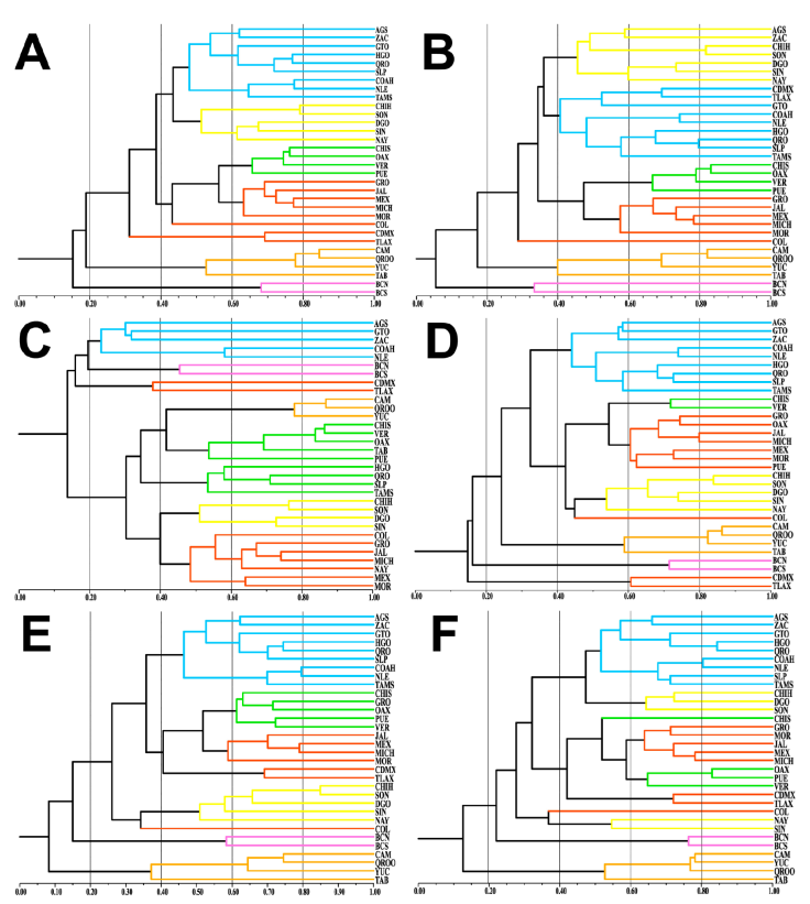
Figure 2 Floristic similarities among Mexican states. A, Total floristic richness; B, Humid Mountain Forest (HMF); C, Humid Tropical Forest (HTF); D, Seasonally Dry Tropical Forest (STF); E, Temperate Forest (TEM); F, Xerophytic Scrub (XER).
Southeastern Mexico (floristic group VI in Table 2) contained the largest number of total species and restricted species. In contrast, the 2 peninsulas had lower richness values, although the Baja California Peninsula (floristic group I) had a significant number of restricted species, comparable to continental regions.
When species richness was segmented by biome, the same general floristic groups were recovered (Fig. 2B-F). Several of these groups remain constant regardless of whether the entire flora or groups of species by biome are analyzed. For example, the floristic composition of group I (Table 2), corresponding to the Baja California Peninsula, was identified chorologically as a cohesive floristic unit in all analyses (Figs. 2, 3). Similarly, the Yucatán Peninsula plus Tabasco (group II) formed a floristic unit in all the analyses, except for HTF species, in which Tabasco was placed with the southeastern states, which had the highest richness in this biome (Figs. 2C, 3C).
Maps by E. Ortiz.
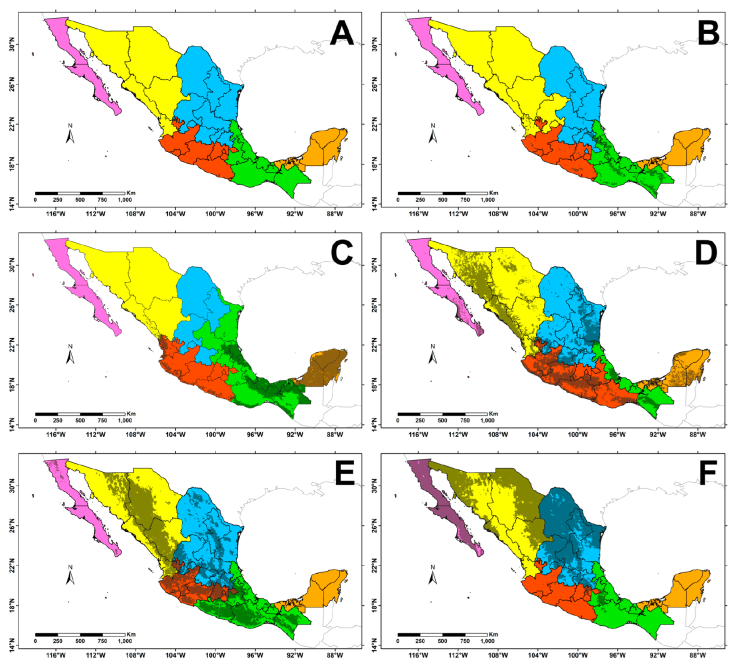
Figure 3 Geographical arrangement of the floristic groups recovered in the cluster analyses (Fig. 2) based on overall floristic richness and richness by biome. A, Total floristic richness; B, Humid Mountain Forest; C, Humid Tropical Forest; D, Seasonally Dry Tropical Forest; E, Temperate Forest; F, Xerophilous Scrub. The gray shading in figures B-F shows the distribution of the corresponding biome.
Figure 3 shows the relationships between the states obtained through the cluster analysis in the geographical space. This representation shows that neighboring states shared a greater number of species, which sorted them into the same floristic group.
Discussion
The first step toward achieving a comprehensive Flora of Mexico is to have a functional and accessible list of species; Villaseñor’s (2016) contribution aimed at this effort. Although the current number of species accepted and that of Villaseñor (2016) is practically identical (Table 1), differences in taxonomic circumscriptions (accepted species) are not shown here. Such differences are mainly the result of the description of new taxa, the revision of taxonomic groups, and other products of taxonomic work that sometimes result in a substantial number of species now considered synonyms, especially when the species are harmonized with the nomenclature accepted by the World Checklist of Vascular Plants (http://wcvp.science.kew.org, Murguía-Romero et al., 2023). Therefore, a review of the list of species that reflect all these taxonomic and nomenclatural changes is needed.
In this work, we present an update of the figures published more than 7 years ago (Villaseñor, 2016), and evaluate changes in floristic composition at the state level (Table 1). Although the use of political divisions is not the most recommended for the analysis of richness and diversity per se, they are important because currently in Mexico, political boundaries define the basis and scope of most conservation decisions, which is one of the main uses of floristic information. The results shown here do not constitute a measurement of the real species distribution; a species can be recorded in a state only in a small fraction of its territory. Consequently, occurrence in each state only reflects their distribution across Mexican territory. More precise assessments of species distribution at the within-state level will reflect additional patterns of richness and distribution at more local scales (see for example Villaseñor et al., 2022, 2023).
Table 1 shows that the hierarchical placement of the states has not changed compared to the figures published by Villaseñor (2016). The 10 richest states in this study were the same as in Villaseñor (2016); the only change was the number of species recorded. On average, more than 400 species have been added to each state inventory since 2016, although 14 states show figures below this average. Several states have a better knowledge of their flora (for example, Mexico City or the states of the Baja California and Yucatán peninsulas); this can be inferred by the fewer new species described and added as new records. In contrast, states like Durango and Puebla record many additions to their inventory, several of them constituting recently described species. It is necessary to have more precise analyses at the state level to know the addition rates of both new species and new records to its flora.
Richness by biome. The occurrence of species among states responds to their biome fidelity; the more widely represented the biome in the state, the broader the species’ distribution (Fig. 3). The richness of species by state and region is associated with the diversity of existing habitats (heterogeneity), as well as their latitudinal position. The greater environmental heterogeneity observed in Chiapas, Oaxaca, and Veracruz, which are located at lower latitudes than Chihuahua, Coahuila, and Sonora, is undeniable. This heterogeneity helps to explain the greater species richness in the former than in the latter.
The use of political states as units of study provides valuable information to begin to understand differences in richness and the probable causes of such inequality (Table 1). For example, there are more biomes in the states of Chiapas and Oaxaca than in Campeche or Chihuahua. In the first 2, there are large areas of humid forests, both lowland (HTF) and mountain (HMF), forming a colorful mosaic where they mix with other biomes, which helps to explain their important species richness. Meanwhile, Campeche and Chihuahua contain fewer biomes, and although they have important floristic richness, their distribution is more homogeneous, forming broad and continuous patches; this explains their lower species richness.
Floristic similarities. We observe congruence between the geographic proximity of states and their floristic similarities, supporting our initial postulate, regardless of whether the analysis considered total richness or was divided by biome. A similar analysis 2 decades ago showed similar results (Espinosa-García et al., 2004). Since then, the floristic cohesiveness of the peninsulas of Baja California and Yucatán (including Tabasco) has been apparent. The differences in the classification of some states between the 2 studies are indicative of the poor floristic knowledge available a couple of decades ago. For example, in that study, Nayarit and Sinaloa were grouped with states located along the Pacific slope, but currently form a floristic group that is more closely related to the northwestern states. The floristic sampling of both states 2 decades ago was biased toward the Pacific slope, especially in the municipality of Culiacán in Sinaloa (Vega-Aviña, 2002), and around the influence of the Aguamilpa hydrological project in Nayarit (Téllez-Valdés, 1995), which mainly covered tropical regions of that slope. Currently, the floras of both states are better known, with much more exploration in their mountainous regions, where the influence of the Sierra Madre Occidental shows greater floristic similarity with the northwestern states of the country.
The identified floristic groups (Figs. 2, 3) share a particular floristic composition, with a significant number of species restricted to their territory (Table 2). Once the flora of each floristic unit is known, it is possible to carry out other analyses considering the set of species that characterizes each one. For example, 3,967 species (out of 14,673) are only known from floristic group VI (Table 2); Oaxaca is first for total floristic richness, but Chiapas slightly surpasses it in exclusive species (2,316 in Chiapas, 2,255 in Oaxaca). If we consider the proportions of exclusive species by state relative to the total in the region, Chiapas contains 58%, Oaxaca 56%, Veracruz 30%, and Puebla 14%. However, although Chiapas and Oaxaca show similar proportions of restricted species, it is interesting to note that only 961 of them are shared (24% of the total), suggesting a high species turnover from one state to the other (i.e., high beta diversity). Species shared between these 2 states include Clethra pachecoana Standl. & Steyerm., Dendrosida breedlovei Fryxell, Saurauia matudae Lundell, Senegalia mirandae (L. Rico) Seigler & Ebinger, and Triplaris melaenodendron (Bertol.) Standl. & Steyerm.
The same exercise in floristic group II, which has only 171 exclusive species, shows that 70% are found in Quintana Roo, 65% in Yucatán, 57% in Campeche, and 15% in Tabasco. Eighty-six species are shared between Quintana Roo and Yucatán (50% of the total), which suggests lower beta diversity compared to group VI. The species shared between Quintana Roo and Yucatán include Harpalyce yucatanense Miranda ex São-Mateus & M.Sousa, Morisonia quintanaroensis (Iltis & Cornejo) Christenh. & Byng, Macroscepis yucatanensis Morillo, Ruellia macrophylla Vahl, Manfreda petskinil R.A.Orellana, L.Hern. & Carnevali, and Wittmackia mesoamericana (I.Ramírez, Carnevali & Cetzal) Aguirre-Santoro. The greater beta diversity in floristic group VI compared to group II suggests higher environmental heterogeneity in the former, which implies a more restricted distribution of its exclusive species than in the latter.
The combination of data from available databases and the use of multivariate techniques currently allow for more robust, refutable, and less intuitive analyses (Kreft & Jetz, 2010). Likewise, the consistent use of the same coefficient in different studies will maximize their comparability, and therefore our understanding of floristic patterns and other ecological attributes (Vellend, 2001). This allows a better knowledge of the geographical distribution of the species and the identification of species assemblages or floristic groups (Table 2), as well as the species characterizing them (floristic elements). Without a doubt, the results obtained in this way will facilitate their use in other lines of research, such as historical biogeography and conservation. The hierarchical patterns found in this study, despite using political divisions, seem to define clear floristic regions, supported even by quite a few exclusive species.
Mexico has a long tradition of interest in floristics. Thanks to this, we currently have a good knowledge of our plant diversity at a national and state level. However, recent explorations and advances in plant systematics strongly highlight the need to periodically synthesize discoveries and changes. This work focused on updating the data on floristic knowledge in each of the states and on analyzing the floristic similarities between them. The data provided here highlight the importance of good floristic knowledge at the regional level, the role played by inventories at the state level, and the botanists involved in their compilation.

